Dijkstra's algorithm

Dijkstra's algorithm finds the shortest distance from one vertex to every other vertex in a graph whose edges have lengths that are not negative, such as a map of roads. If every step costs the same, as in a maze, BFS is simpler; if some lengths are negative, use Bellman–Ford.

Explanation

For example, a town has 4 junctions (vertices) and 4 two-way roads (edges), and each road has a length (its weight). Find the shortest route from junction 1 to junction 4.

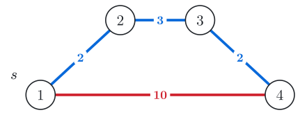
Fig. 1. The direct road to junction 4 has length 10. The route through junctions 2 and 3 uses three roads and has length 7.

Look at junction 4. The red road leads straight there from junction 1, but its length is 10. The blue route through junctions 2 and 3 uses three roads and has length 2 + 3 + 2 = 7. The shortest path is not always the one with the fewest roads. In this example it's easy to see which route is shorter, but in a bigger town there are many routes to compare, and we need a method that finds the best one without trying them all.

A bigger town has 6 junctions and 9 roads, and we look for the shortest route from junction 1 to junction 5.

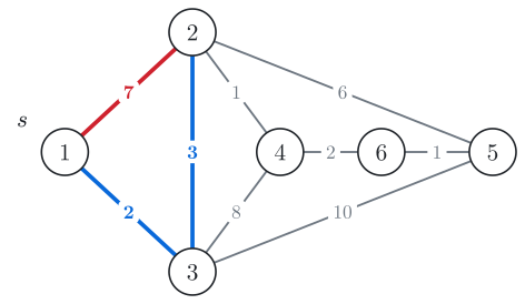
Fig. 2. Find the shortest route from junction 1 to junction 5. Junction 2 is first reached along the red road (7). The blue route through junction 3 is shorter (5).

The natural first idea is to spread out from junction 1: visit its neighbours, then their neighbours, and write next to each junction the length of the route it was reached by. Junction 2 is reached along the red road, so it gets 7. But the blue route through junction 3 is 2 + 3 = 5. If we keep the first length we find, junction 2 stays at 7, which is not the shortest.

Instead, we can keep the smallest length found so far: whenever a shorter route to a junction turns up, we replace its number and visit it again, because its neighbours may now be closer too. This gives the right answer, but it repeats work. Junction 2 is visited twice: first with 7, then again with 5, and every road out of it is checked both times. In a bigger town one junction can be revisited many times, and each revisit spreads to its neighbours.

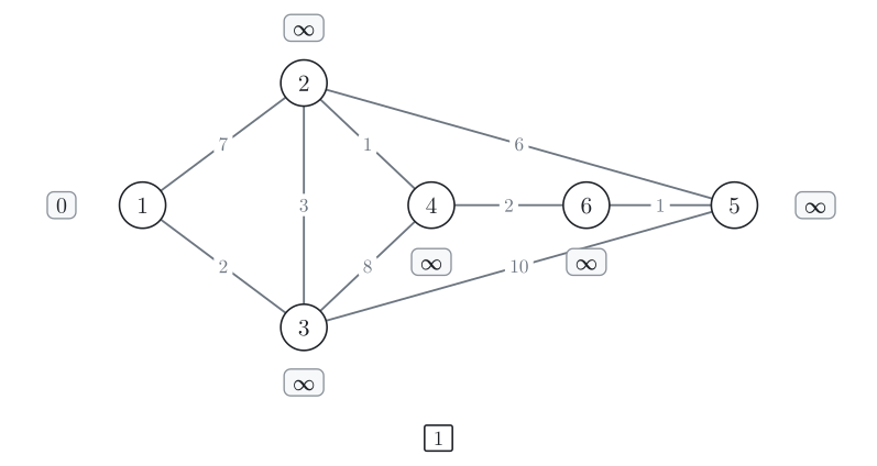
Junction 1 gets the number 0 and waits to be visited.

Junction 1 is visited, with the number 0. Visit 1.

The road from junction 1 gives junction 2 the number 7, and junction 2 waits to be visited.

The road from junction 1 gives junction 3 the number 2, and junction 3 waits to be visited.

Junction 2 is visited, with the number 7. Visit 2.

The road from junction 2 to junction 1 gives 14, no better than its number 0. Nothing changes.

The road from junction 2 to junction 3 gives 10, no better than its number 2. Nothing changes.

The road from junction 2 gives junction 4 the number 8, and junction 4 waits to be visited.

The road from junction 2 gives junction 5 the number 13, and junction 5 waits to be visited.

Junction 3 is visited, with the number 2. Visit 3.

The road from junction 3 to junction 1 gives 4, no better than its number 0. Nothing changes.

The road from junction 3 lowers the number of junction 2 from 7 to 5, so junction 2 waits to be visited again.

The road from junction 3 to junction 4 gives 10, no better than its number 8. Nothing changes.

The road from junction 3 lowers the number of junction 5 from 13 to 12, so junction 5 waits to be visited again.

Junction 4 is visited, with the number 8. Visit 4.

The road from junction 4 to junction 2 gives 9, no better than its number 5. Nothing changes.

The road from junction 4 to junction 3 gives 16, no better than its number 2. Nothing changes.

The road from junction 4 gives junction 6 the number 10, and junction 6 waits to be visited.

Junction 5 is visited, with the number 12. Visit 5.

The road from junction 5 to junction 2 gives 18, no better than its number 5. Nothing changes.

The road from junction 5 to junction 3 gives 22, no better than its number 2. Nothing changes.

The road from junction 5 to junction 6 gives 13, no better than its number 10. Nothing changes.

Junction 2 is visited again, with the number 5. Visit 6.

The road from junction 2 to junction 1 gives 12, no better than its number 0. Nothing changes.

The road from junction 2 to junction 3 gives 8, no better than its number 2. Nothing changes.

The road from junction 2 lowers the number of junction 4 from 8 to 6, so junction 4 waits to be visited again.

The road from junction 2 lowers the number of junction 5 from 12 to 11, so junction 5 waits to be visited again.

Junction 5 is visited again, with the number 11. Visit 7.

The road from junction 5 to junction 2 gives 17, no better than its number 5. Nothing changes.

The road from junction 5 to junction 3 gives 21, no better than its number 2. Nothing changes.

The road from junction 5 to junction 6 gives 12, no better than its number 10. Nothing changes.

Junction 6 is visited, with the number 10. Visit 8.

The road from junction 6 to junction 4 gives 12, no better than its number 6. Nothing changes.

The road from junction 6 to junction 5 gives 11, no better than its number 11. Nothing changes.

Junction 4 is visited again, with the number 6. Visit 9.

The road from junction 4 to junction 2 gives 7, no better than its number 5. Nothing changes.

The road from junction 4 to junction 3 gives 14, no better than its number 2. Nothing changes.

The road from junction 4 lowers the number of junction 6 from 10 to 8, so junction 6 waits to be visited again.

Junction 5 is visited again, with the number 11. Visit 10.

The road from junction 5 to junction 2 gives 17, no better than its number 5. Nothing changes.

The road from junction 5 to junction 3 gives 21, no better than its number 2. Nothing changes.

The road from junction 5 to junction 6 gives 12, no better than its number 8. Nothing changes.

Junction 6 is visited again, with the number 8. Visit 11.

The road from junction 6 to junction 4 gives 10, no better than its number 6. Nothing changes.

The road from junction 6 lowers the number of junction 5 from 11 to 9, so junction 5 waits to be visited again.

Junction 5 is visited again, with the number 9. Visit 12.

The road from junction 5 to junction 2 gives 15, no better than its number 5. Nothing changes.

The road from junction 5 to junction 3 gives 19, no better than its number 2. Nothing changes.

The road from junction 5 to junction 6 gives 10, no better than its number 8. Nothing changes.

No junction is waiting any more. The first attempt needed 12 visits for 6 junctions.

1/50

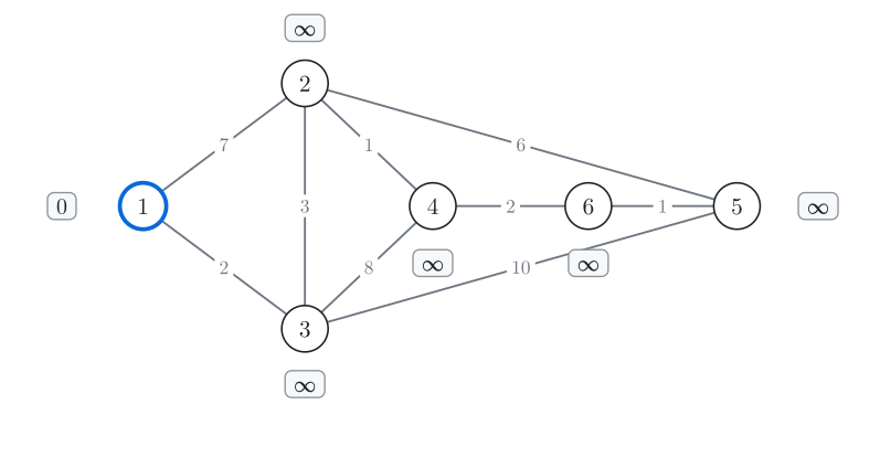
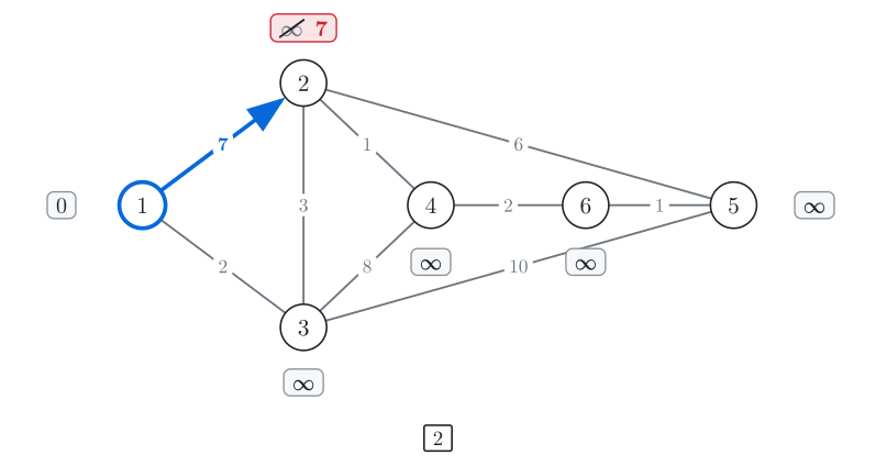
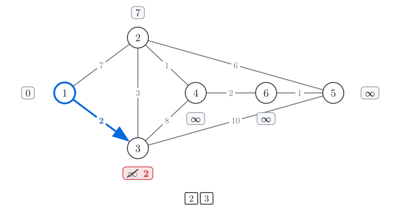
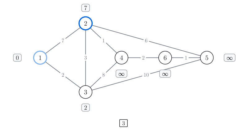
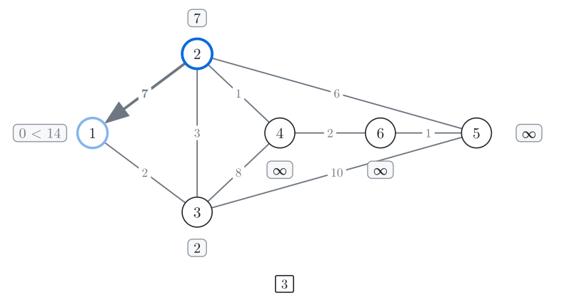
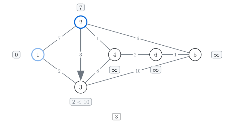
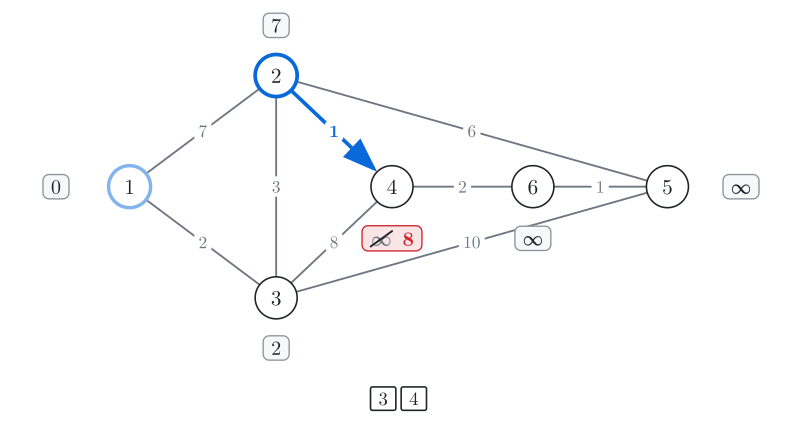
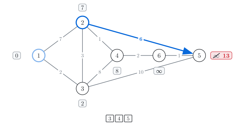
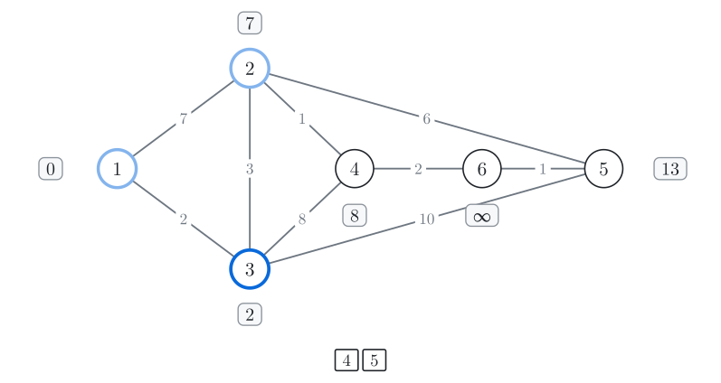
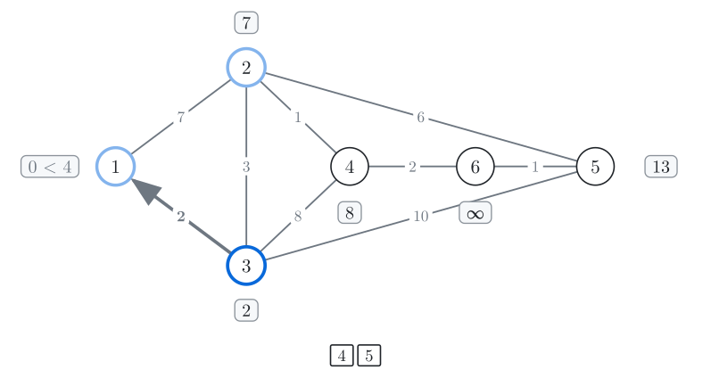
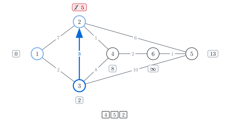
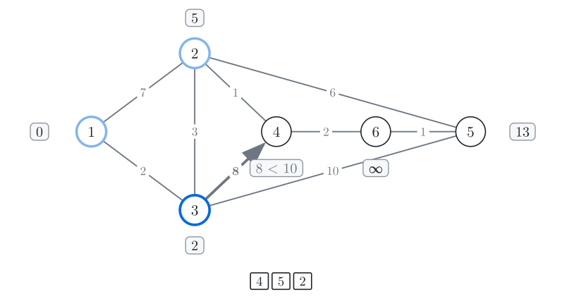
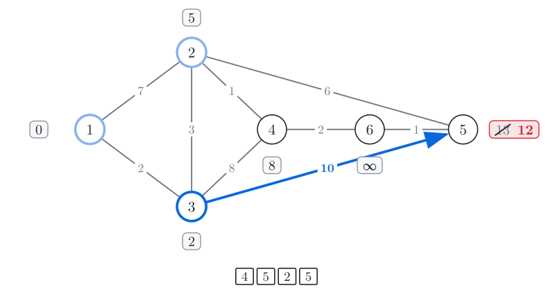
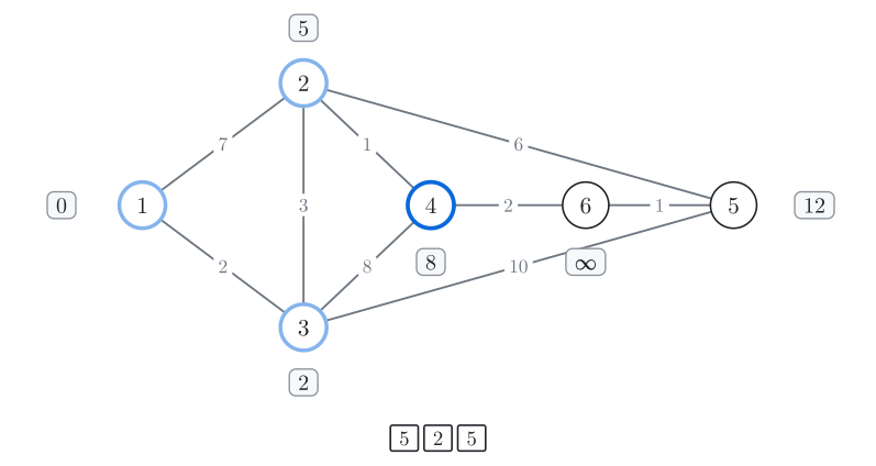
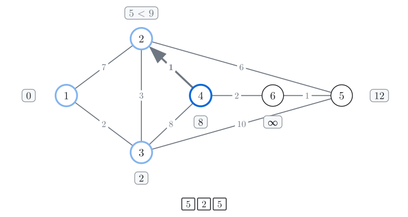
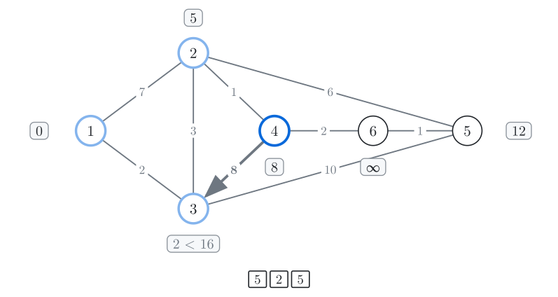
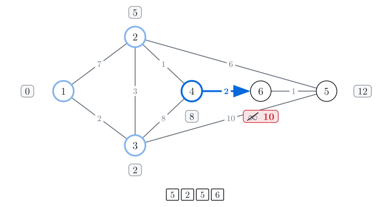
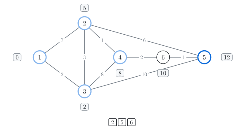
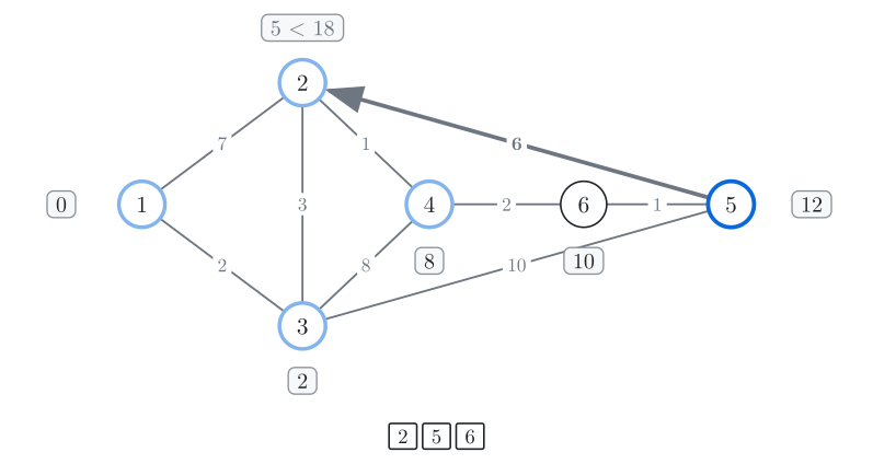
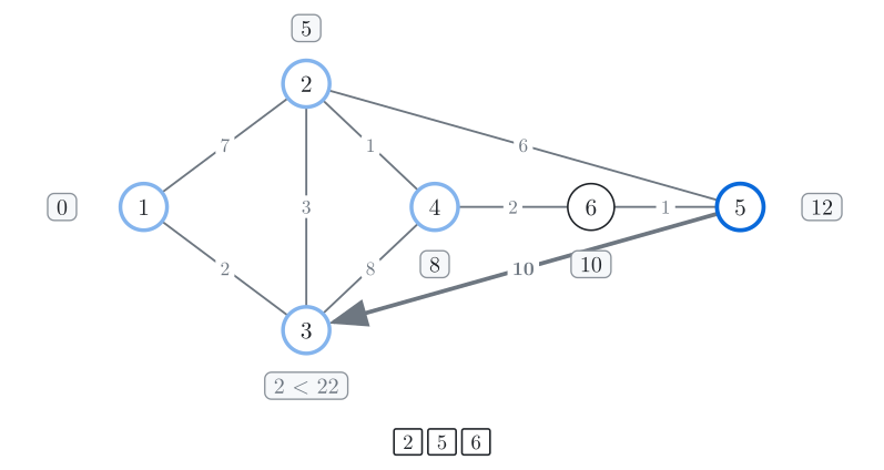
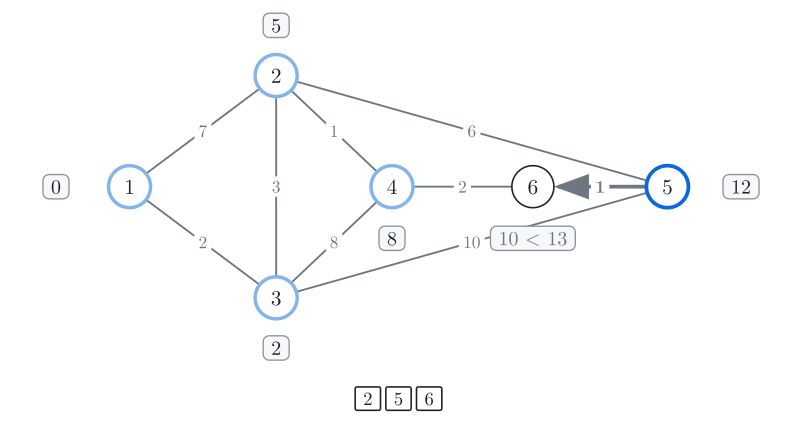
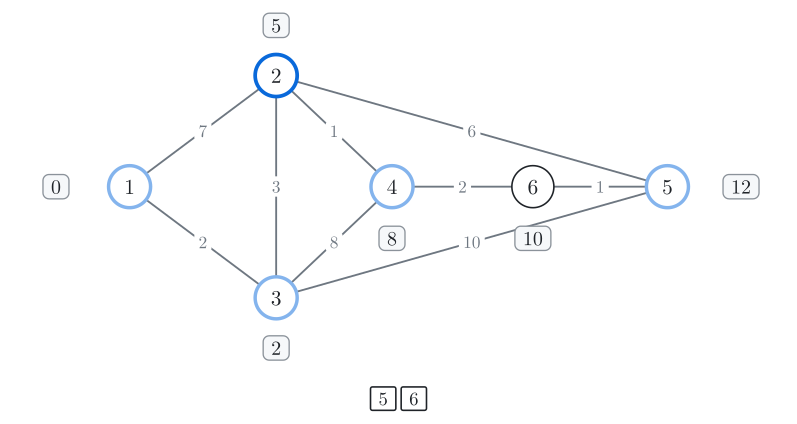
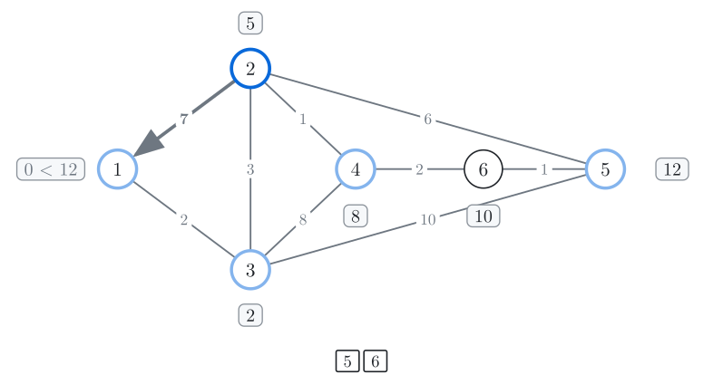
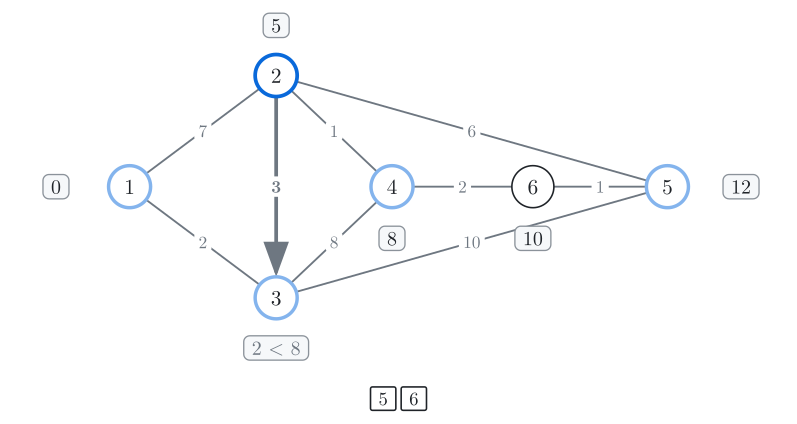
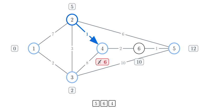
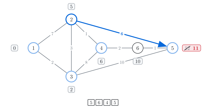
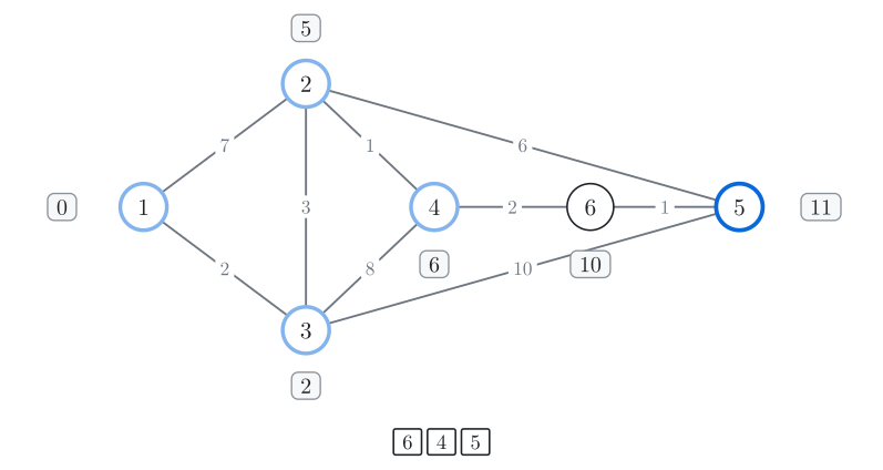
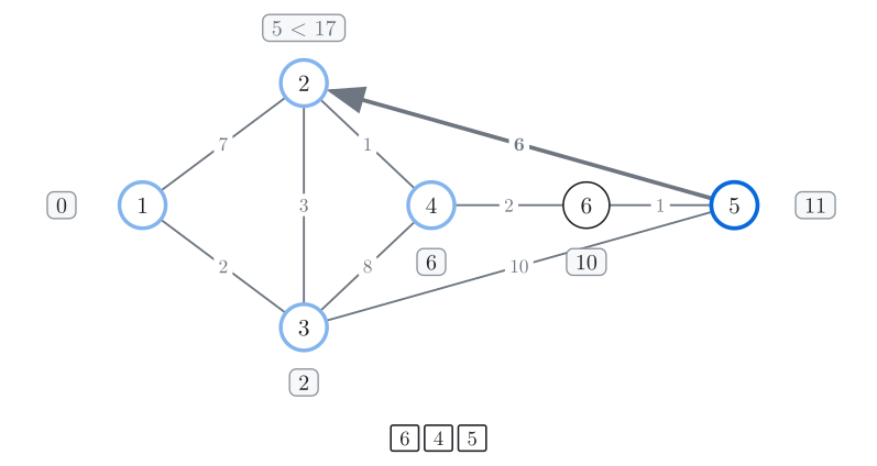
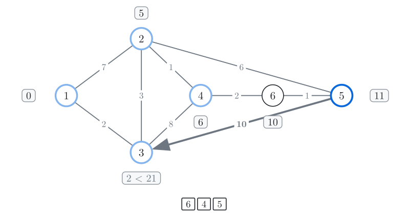
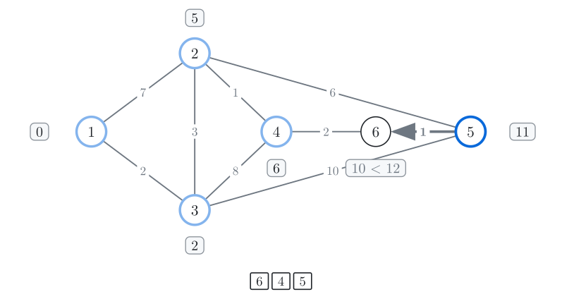
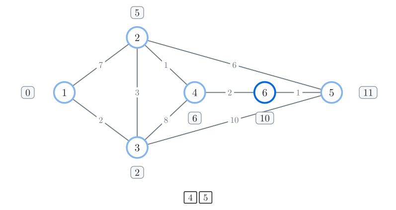
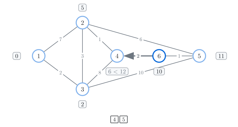
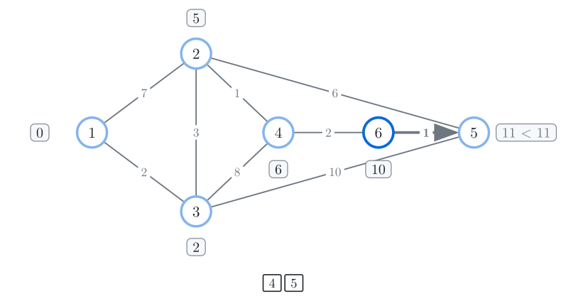
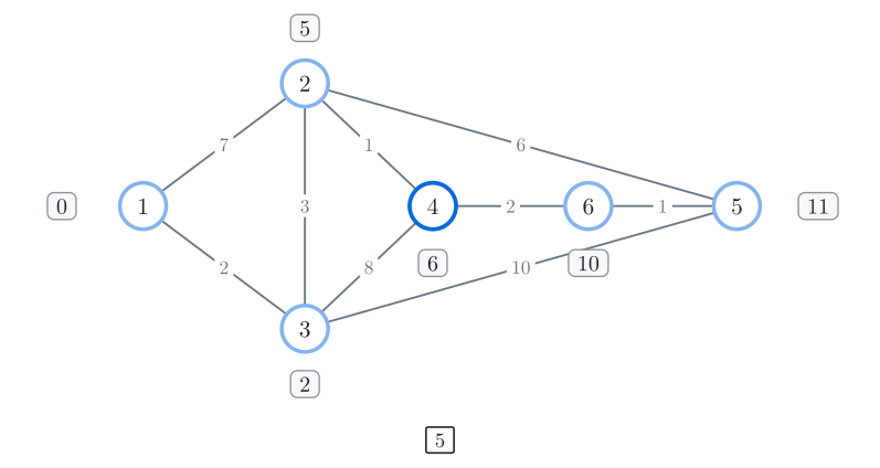
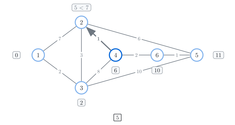
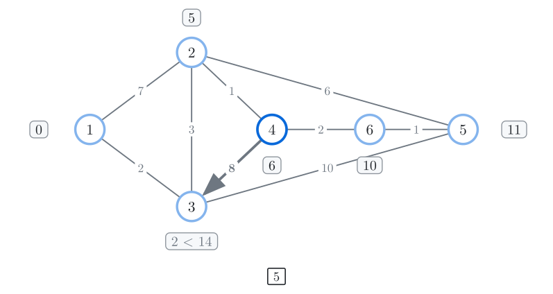
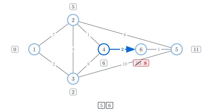
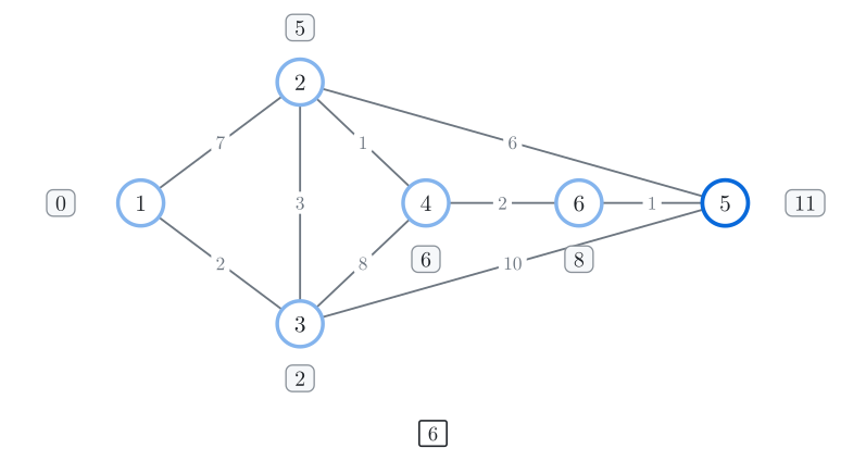
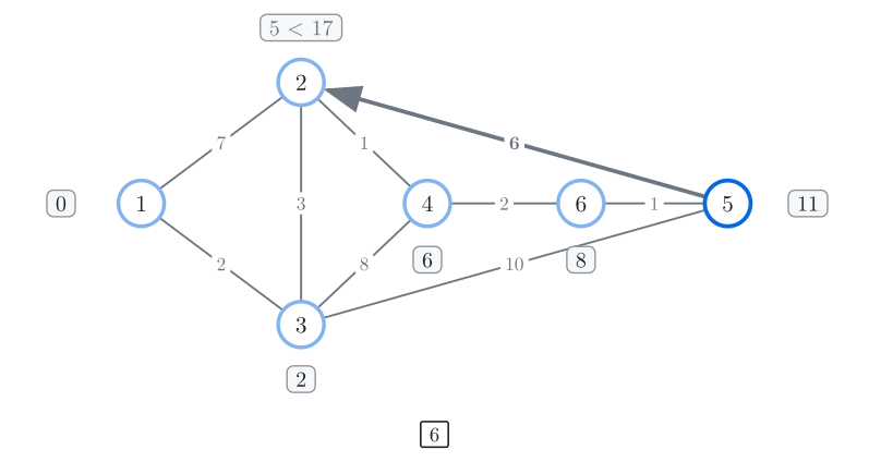
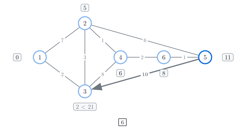
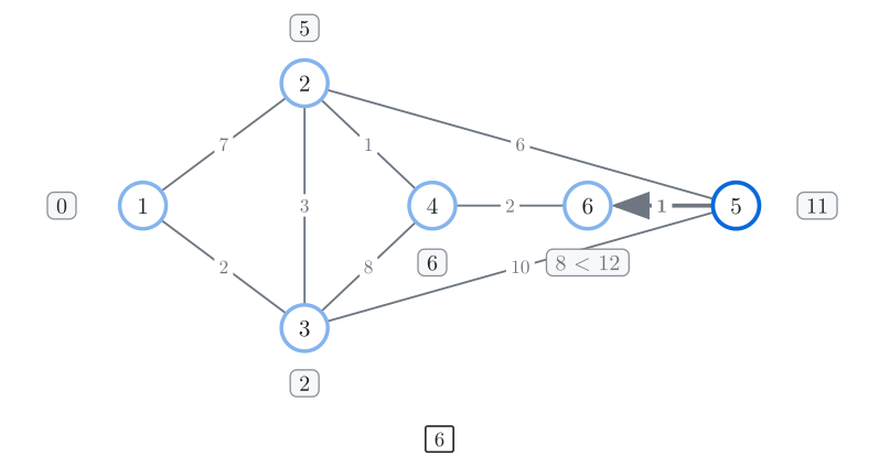
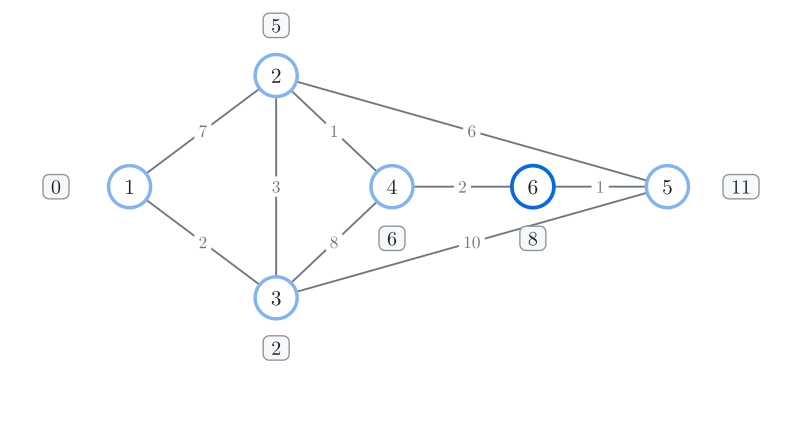
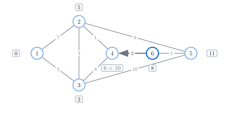
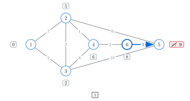
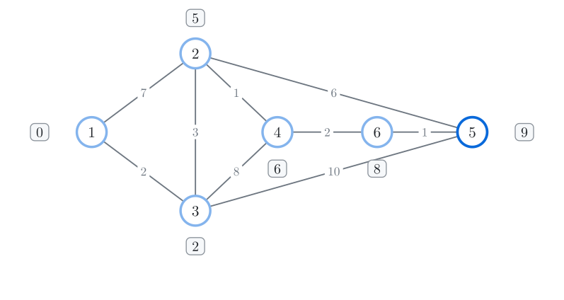
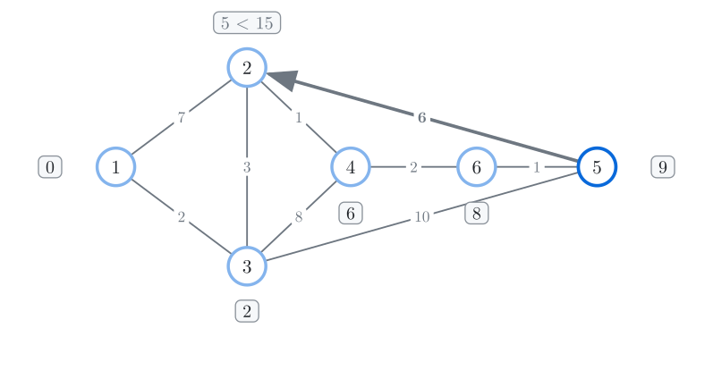
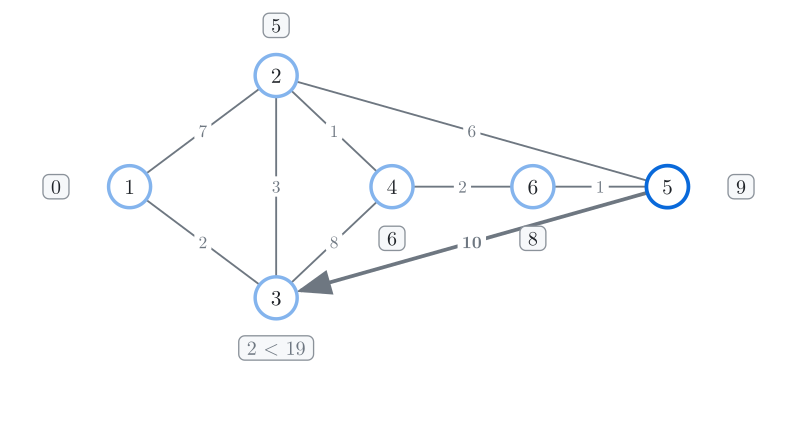
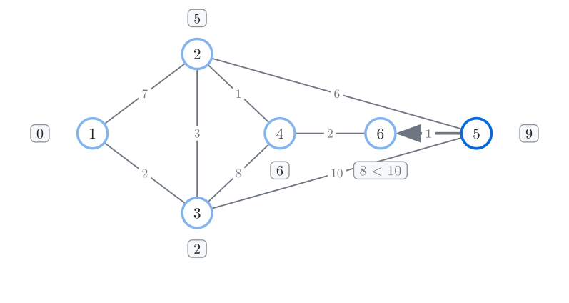
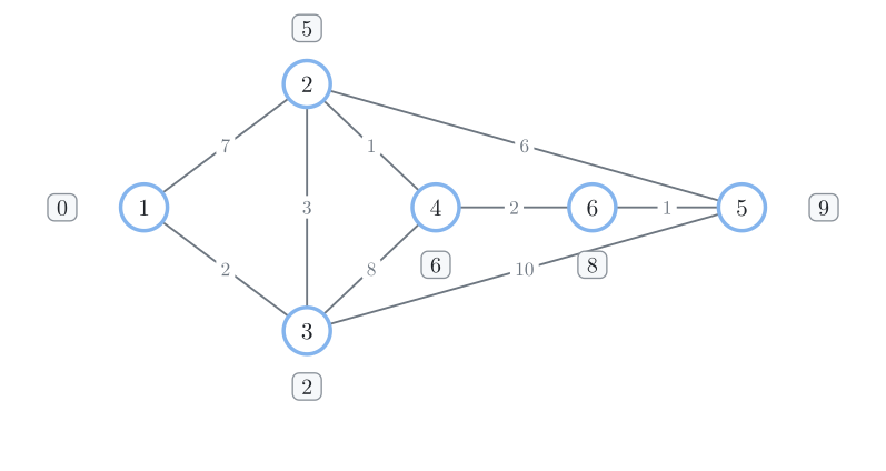
Fig. 3. Step through the first attempt with the buttons. Each step checks one road: a blue arrow improves a number, a grey one doesn't. Light blue junctions have been visited, and the boxes below wait to be visited, next one first. 12 visits for 6 junctions.

The repeats come from visiting junction 2 too early: when we first visited it, its number wasn't final yet. So the question is which order of visiting junctions is optimal. Take the one with the smallest number among those not visited yet. Its number can't get any smaller. Any other route to it has to pass through another junction we haven't visited yet, and that junction is already at least as far away. Lengths are never negative, so the rest of the route can only add to that. In our town, junction 3 (2) is visited before junction 2 (7), and through it junction 2 gets 5 before we ever visit it. Each junction is visited once, with its final distance.

This is Dijkstra's algorithm: always visit the closest junction you haven't visited yet, and use its roads to shorten its neighbours' numbers. Each junction is visited once, and once visited, its number is final.

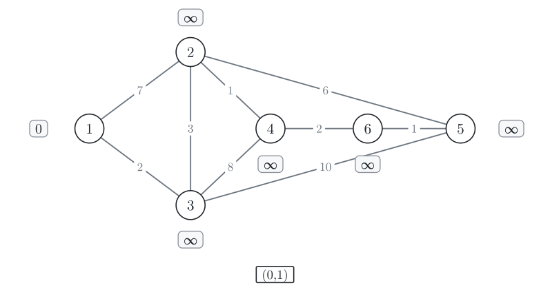
Junction 1 gets the number 0. Every other junction has no number yet.

Junction 1 has the smallest number among the junctions not visited yet, 0. It is visited, and its number is final.

The road from junction 1 gives junction 2 the number 7, and the box (7,2) joins the queue.

The road from junction 1 gives junction 3 the number 2, and the box (2,3) joins the queue.

Junction 3 has the smallest number among the junctions not visited yet, 2. It is visited, and its number is final.

The road from junction 3 lowers the number of junction 2 from 7 to 5, and the box (5,2) joins the queue.

The road from junction 3 gives junction 4 the number 10, and the box (10,4) joins the queue.

The road from junction 3 gives junction 5 the number 12, and the box (12,5) joins the queue.

Junction 2 has the smallest number among the junctions not visited yet, 5. It is visited, and its number is final. The box (7,2) is out of date now and crossed out.

The road from junction 2 lowers the number of junction 4 from 10 to 6, and the box (6,4) joins the queue.

The road from junction 2 lowers the number of junction 5 from 12 to 11, and the box (11,5) joins the queue.

Junction 4 has the smallest number among the junctions not visited yet, 6. It is visited, and its number is final. The box (10,4) is out of date now and crossed out.

The road from junction 4 gives junction 6 the number 8, and the box (8,6) joins the queue.

Junction 6 has the smallest number among the junctions not visited yet, 8. It is visited, and its number is final.

The road from junction 6 lowers the number of junction 5 from 11 to 9, and the box (9,5) joins the queue.

Junction 5 has the smallest number among the junctions not visited yet, 9. It is visited, and its number is final. The boxes (11,5) and (12,5) are out of date now and crossed out.

Every junction has been visited once: 6 visits for 6 junctions, and every number is final.

1/17

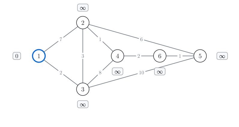
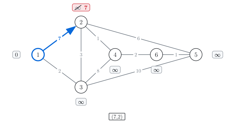
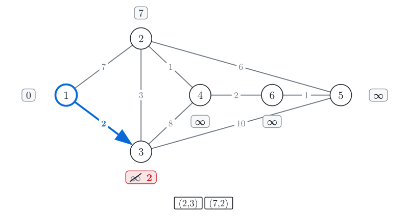
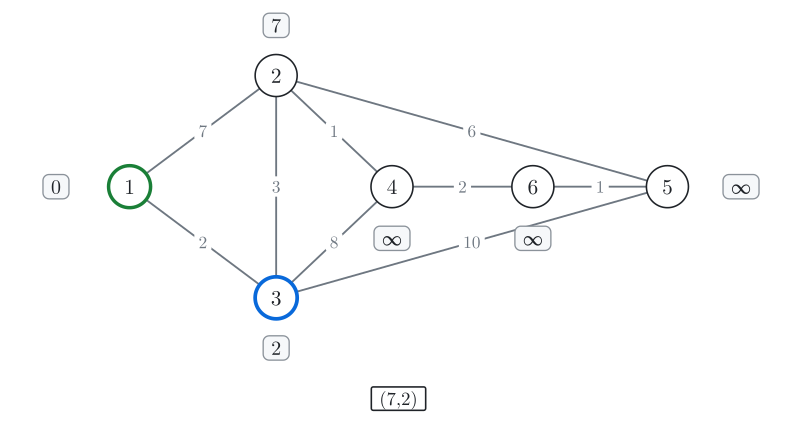
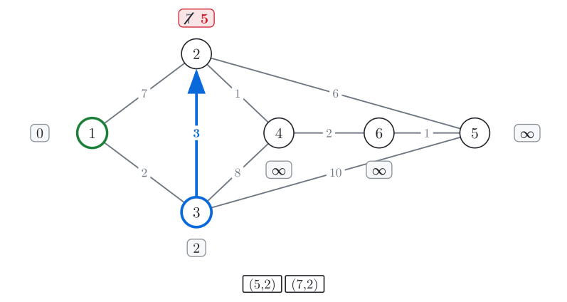
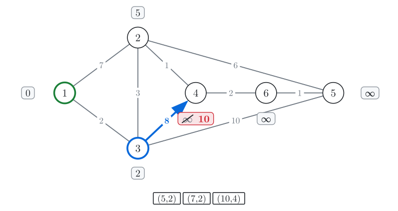
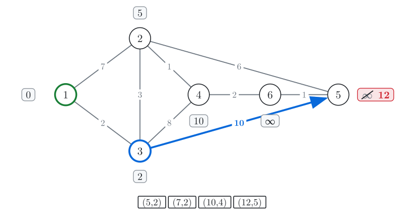
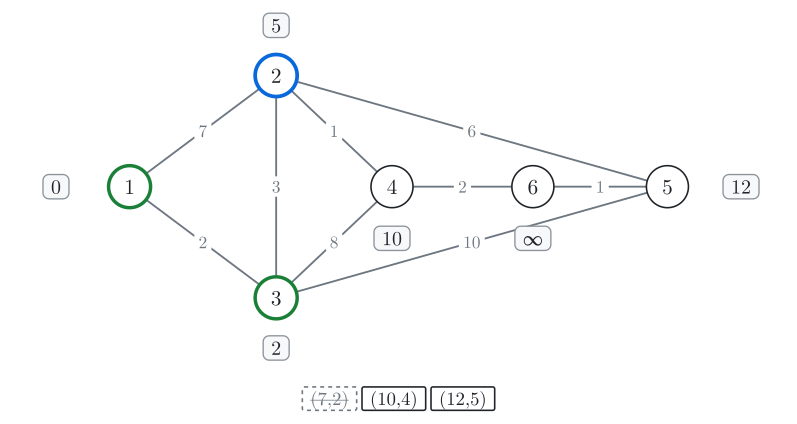
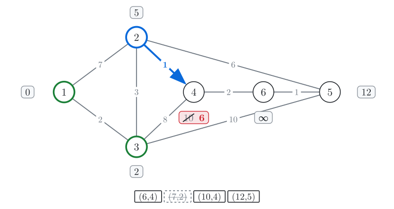
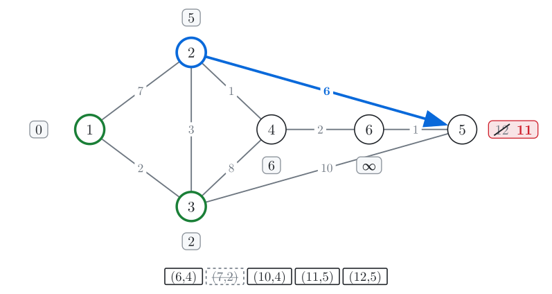
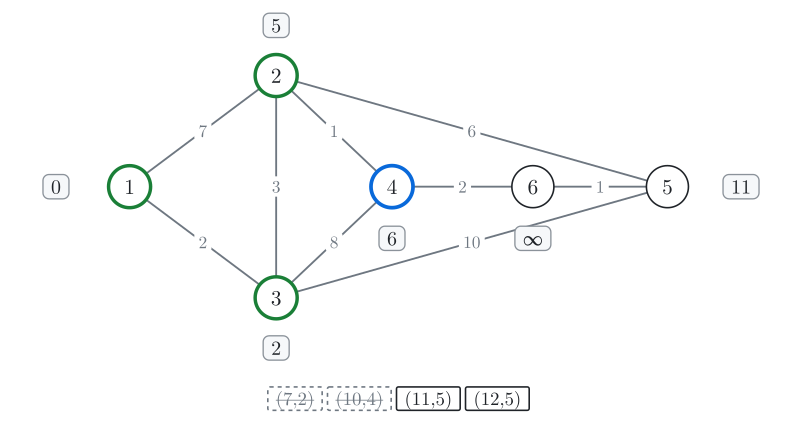
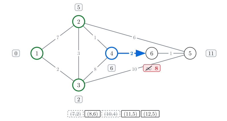
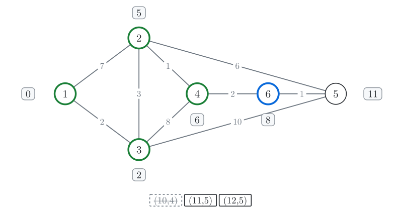
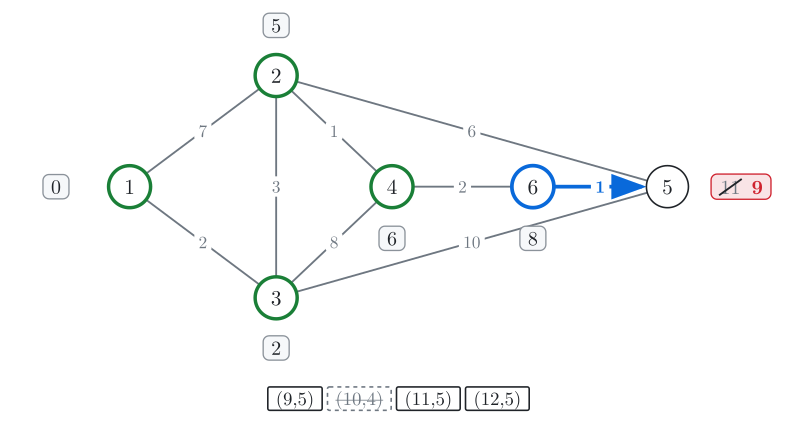
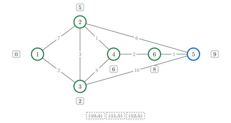
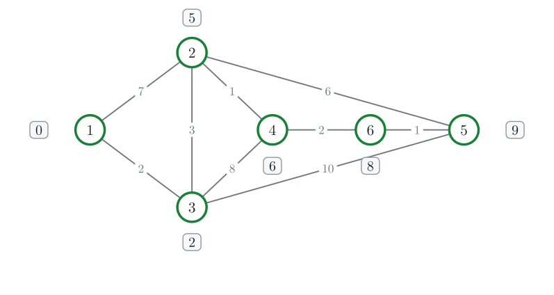
Fig. 4. Step through Dijkstra's algorithm with the buttons. Green junctions have been visited and their numbers are final, and the boxes below are the priority queue. 6 visits for 6 junctions.

The shortest route from junction 1 to junction 5 has length 9. The same run also found the shortest distance from junction 1 to every other junction: 5 for junction 2, 2 for 3, 6 for 4, 9 for 5 and 8 for 6. It visited each junction once: 6 visits, against 12 for the first attempt.

Implementation

Let's keep the distances in an array dist: dist[v] is the length of the shortest route from the starting vertex s to v found so far. At the start dist[s] = 0, and every other value is INF, a number larger than any real distance. When v is visited, dist[v] is final, and we call v processed.

When we visit v, we check each of its roads to a vertex u, of length w. If dist[v] + w < dist[u], the route through v is shorter, and we set dist[u] = dist[v] + w. This check is called relaxing the road.

To find the closest unvisited vertex quickly, we keep the vertices waiting to be visited in a priority queue of pairs (distance, vertex), which always gives out the pair with the smallest distance. These are the boxes under the map in Fig. 4. When dist[u] improves, we push a new pair (dist[u], u). The old pair for u stays in the queue, because std::priority_queue can't change a pair that is already inside. When an old pair comes out, its distance no longer matches dist[u], because u was already processed with a smaller one, so we skip it; such a pair is called stale. In Fig. 4, (7,2) stays in the queue after junction 2 gets 5, and is skipped later.

For a starting vertex s, the algorithm is:

1. Initialise: dist[s] = 0, every other dist[v] is INF, and the queue holds (0, s).

2. Take the smallest pair (d, v). If d != dist[v], the pair is stale: skip it. Otherwise v is processed now, and dist[v] is final.

3. Relax every edge of v, and push (dist[u], u) for each one that improves.

4. Repeat from step 2 until the queue is empty.

If you only need the distance to one target t, you can stop as soon as t is processed.

The program reads n and m, then m lines u v w: a road between u and v of length w. It prints the distance to each vertex, or -1 for a vertex that can't be reached, and then the shortest path from vertex 1 to vertex n. The path is kept in an array parent: parent[u] is the vertex whose edge last improved dist[u], and walking back along it from n reaches vertex 1. For the 6-junction town the input is:

6 9
1 2 7
1 3 2
2 3 3
2 4 1
2 5 6
3 4 8
3 5 10
4 6 2
5 6 1

The graph is stored as an adjacency list g of (neighbour, weight) pairs; g and dist are indexed by vertex from 1 to n. The pair taken from the queue is unpacked into its distance d and its vertex v, and d != dist[v] is the stale check of step 2. N5 and INF are small here so that the trace is easy to follow; for real inputs, use the values in the comments. The pair in the priority queue is (distance, vertex). std::priority_queue is a heap that gives out the largest element, and greater<> makes it give out the smallest pair first.

#include <bits/stdc++.h>
using namespace std;

#define ll long long

const ll N5 = 7;     // small for the demo; use 2e5 + 7 for real inputs
const ll INF = 99;   // small for the demo; use 4e18 for real inputs
vector < pair<ll,ll> > g[N5];

ll dist[N5];
int parent[N5];   // only needed to print the path

void dijkstra(int n, int start){

    for (int i = 1 ; i<=n ; i++) dist[i] = INF;

    priority_queue<pair<ll, int>, vector<pair<ll, int>>, greater<pair<ll, int>>> pq;

    dist[start] = 0;
    pq.push({0, start});

    while (!pq.empty()) {
        auto [d, v] = pq.top();
        pq.pop();

        if (d != dist[v]) continue;

        for (auto [u, w] : g[v]) {
            if (dist[u] > dist[v] + w) {
                dist[u] = dist[v] + w;
                parent[u] = v;   // only needed to print the path
                pq.push({dist[u], u});
            }
        }
    }

}

int main() {
    ios::sync_with_stdio(0);
    cin.tie(0);

    int n, m;
    cin >> n >> m;

    for (int i = 0; i < m; i++) {
        int u, v;
        ll w;
        cin >> u >> v >> w;
        g[u].push_back({v, w});
        g[v].push_back({u, w});   // remove this line if the graph is directed
    }

    dijkstra(n , 1);

    for (int i = 1; i <= n; i++) {
        cout << (dist[i] == INF ? -1 : dist[i]) << " ";
    }
    cout << "\n";

    // print the shortest path from 1 to t; remove this block if you only need distances
    int t = n;
    if (dist[t] != INF) {
        vector<int> path;
        for (int v = t; v != 0; v = parent[v]) path.push_back(v);
        reverse(path.begin(), path.end());
        for (int v : path) cout << v << " ";
    }
}

Each edge is relaxed once from each processed end and pushes at most one pair, so the priority queue receives at most 2m + 1 pairs, each pushed and taken in O(\log m). The time is O((n + m) \log m), often written O((n + m) \log n) since m \le n^2, and the memory is O(n + m).

For a graph with close to n^2 edges, given as an n \times n table of weights (an adjacency matrix), with $n$ up to a few thousand, you can drop the priority queue. Each step scans all $n$ vertices for the unprocessed one with the smallest dist[v], which takes O(n^2) in total. For n = 5000 that is 2.5 \cdot 10^7 operations, against about 3 \cdot 10^8 for the version above.

Correctness proof

The algorithm keeps this invariant: when a vertex is taken from the priority queue and the pair is not stale, its tentative distance equals the length of its shortest path from the source.

The source is taken first with d_s = 0, which is correct. Every finite d_v is the length of some path, because it was set by a relaxation along a real edge, so d_v is never too small. Now suppose a vertex v \ne s is taken with distance d_v, and all vertices processed before it have correct distances. Take any path $P$ from $s$ to $v$. It starts at a processed vertex and ends at an unprocessed one, so it has a first unprocessed vertex $y$, and the vertex $x$ just before $y$ on $P$ is processed. When $x$ was processed, the edge $x$–$y$ was relaxed, so d_y is at most the length of $P$ up to $y$, and some pair (d_y, y) is in the priority queue. The pair of $v$ was taken first, so d_v \le d_y. The rest of $P$, from $y$ to $v$, has non-negative edges, so the length of $P$ is at least d_y \ge d_v. No path to $v$ is shorter than d_v. In the example, when v = 4 is taken with d_4 = 6, the path 1 → 3 → 5 → 6 → 4 leaves the processed vertices at y = 5, and d_5 = 11 \ge 6.

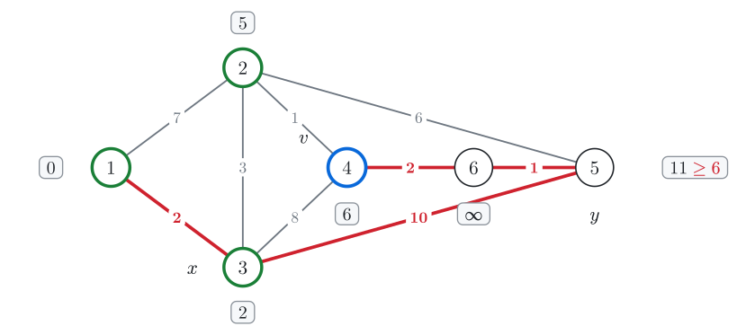
Fig. 5. The green vertices are processed, and v = 4 is being taken with d_v = 6. The red path $P$ leaves the processed vertices at y = 5, where d_y = 11 \ge 6, and the edges after $y$ can only add length.

Negative weights

The proof used one fact: the part of $P$ after $y$ can't have negative length. With a negative edge this fails. Edges of weight 0 are allowed.

Take a directed graph with edges 1→2 (2), 1→3 (3), 3→2 (−2) and 2→4 (2), source 1. The true distances are [0, 1, 3, 3], because 1 → 3 → 2 → 4 has length 3 − 2 + 2 = 3.

Dijkstra takes vertex 1, then vertex 2 with distance 2, and relaxes 2→4 to set d_4 = 4. Then it takes vertex 3 with distance 3. The edge 3→2 lowers d_2 to 1, but vertex 2 is already processed, so its edges are never relaxed again and d_4 stays 4. The output is 0 1 3 4, and d_4 is wrong.

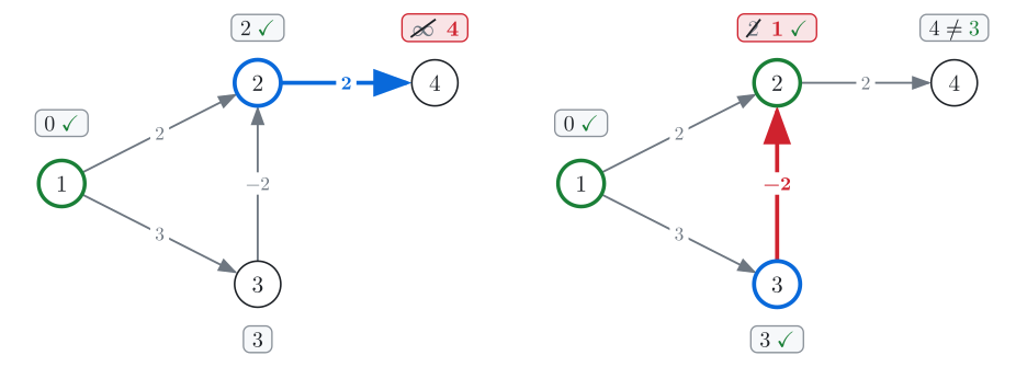
Fig. 6. Vertex 2 was processed before the negative edge 3→2 was seen, so the shorter path to vertex 4 is never found.

With the weight of 3→2 set to −1, the output 0 2 3 4 happens to be correct. A negative edge doesn't always break the answer, but nothing guarantees a correct one either. Bellman–Ford allows negative edges and runs in $O(nm)$. It also detects negative cycles.

Common mistakes

• Marking a vertex processed when it is pushed, as BFS does, so a vertex keeps the first distance it gets and a shorter route found later is rejected. Dijkstra must mark a vertex when it is taken from the queue.

• Taking the largest pair first, as priority_queue<pair<ll, int>> does without greater<>. Use priority_queue<P, vector<P>, greater<P>>, or push negated distances.

• Not skipping stale pairs, so every pair taken relaxes its vertex's edges again: the answers stay correct, but a vertex with 10^5 edges can cost 10^{10} relaxations. Keep if (d != dist[v]) continue;.

• Adding a constant to remove negative weights, which changes which path is shortest, because a path with more edges gains more. Use Bellman–Ford for negative weights.

Similar algorithms

The first attempt at the top of this article, spreading out from the start, is BFS. It gives correct distances when every edge has the same weight. Dijkstra on such a graph processes the vertices in BFS order but pays an extra log factor, so first check whether the edges really have different weights.

When some weights are negative, use Bellman–Ford, which runs in $O(nm)$.

When every weight is 0 or 1, 0-1 BFS replaces the priority queue with a deque and runs in O(n + m).

Prim's algorithm has almost the same loop with a priority queue, so the two are often confused. In Prim, the key of a vertex is the weight of one edge, not the length of a path. The result is a minimum spanning tree, the cheapest set of edges that connects all vertices, not shortest distances.

When the cost depends on more than the current vertex, such as fuel left or the step number modulo 3, run Dijkstra on a state graph whose vertices are pairs (place, state).

Practice