Prim's algorithm

Prim's algorithm finds a minimum spanning tree of an undirected weighted graph: the cheapest set of edges that connects all its vertices. If you need the shortest routes from one vertex instead, use Dijkstra's algorithm.

Explanation

A district has 4 villages joined by dirt roads, and paving each road costs a known amount. We want to pave some roads so that we can drive between any two villages on paved roads, and spend as little as possible.

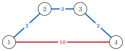
Fig. 1. The four roads form one loop.

One road of a loop is never needed: without it, the villages on the loop are still connected the other way round. So we leave out the dearest road, 1–4, and pave the other three for 2 + 3 + 2 = 7. The paved roads have no loop left, and 4 villages need exactly 3 roads.

The three paved roads are also the shortest routes from village 1. To village 4, the route over the top costs 7, less than the direct road at 10.

A bigger district has more loops, and they share roads.

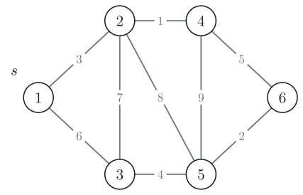
Fig. 2. Pave roads so that every village can be reached, as cheaply as possible.

The small loops here are 1–2–3, 2–3–5, 2–4–5 and 4–5–6. Dropping the dearest road of each one (the roads that cost 7, 8 and 9) still leaves a loop around the whole map, through all six villages. Drop its dearest road too, the 6, and we pay 15. This works, but every drop needs a search for a loop first. A map with 100 000 villages and 200 000 roads needs about 100 000 roads dropped, and each search walks the whole map, about 300 000 steps. That is 30 000 000 000 steps in total, far too slow.

On the small map, the paved roads were the shortest routes from village 1. Dijkstra's algorithm finds those in one pass. Every village except village 1 gets exactly one road, the last road of its shortest route, so these roads reach every village and leave no loop to drop. Let's pave those roads. That gives five roads and a total of 3 + 6 + 1 + 4 + 5 = 19.

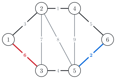
Fig. 3. The roads of the shortest routes from village 1 cost 19.

Look at the red road (6). It gives village 3 a short route from village 1. But if we pave the blue road (2) instead, village 3 is still reached, through villages 6 and 5, and the total drops to 15. A village needs only one paved road to a village already joined to village 1.

Let's grow the joined part from village 1. Next to each village outside it, write the cost of its cheapest road to a joined village. Then join the village with the smallest number, by that road. This is never a mistake. Take any plan that reaches every village, and add to it the cheapest road out of the joined part. That road closes a loop, and the loop has to cross between the joined villages and the others a second time, by another road. Remove that other road: every village is still reached, and the plan gets no dearer. On our map, when villages 1, 2, 4 and 6 are joined, the cheapest road out is the blue one. Added to the plan of Fig. 3, it closes a loop that crosses back by the red road, and removing the red road is the swap above.

This is Prim's algorithm. The paved roads form a minimum spanning tree: roads with no loop that reach every village, at the smallest total cost. Each step is Dijkstra's step, with the cost of one road in place of the distance from the start.

Here is the whole run on the map of Fig. 2. The boxes below the map are pairs (number, village) waiting in a priority queue, as in Dijkstra.

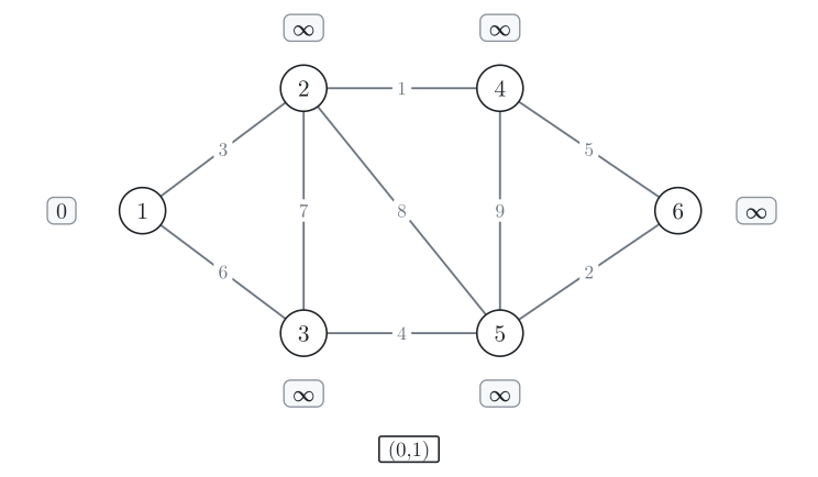
Village 1 gets the number 0, and the box (0,1) waits in the queue. Every other village has ∞.

Village 1 has the smallest number, 0, so it joins first. The total is 0.

The road from village 1 to village 2 costs 3, so village 2 gets the number 3, and the box (3,2) joins the queue.

The road from village 1 to village 3 costs 6, so village 3 gets the number 6, and the box (6,3) joins the queue.

Village 2 has the smallest number outside the tree, 3, so it joins by the road 1–2. The total is 3.

The road from village 2 to village 4 costs 1, so village 4 gets the number 1, and the box (1,4) joins the queue.

The road from village 2 to village 5 costs 8, so village 5 gets the number 8, and the box (8,5) joins the queue.

Village 4 has the smallest number outside the tree, 1, so it joins by the road 2–4. The total is 4.

The road from village 4 to village 6 costs 5, so village 6 gets the number 5, and the box (5,6) joins the queue.

Village 6 has the smallest number outside the tree, 5, so it joins by the road 4–6. The total is 9.

The road from village 6 to village 5 costs 2, less than its number 8, so village 5 gets the number 2, and the box (2,5) joins the queue.

Village 5 has the smallest number outside the tree, 2, so it joins by the road 6–5. The total is 11.

The road from village 5 to village 3 costs 4, less than its number 6, so village 3 gets the number 4, and the box (4,3) joins the queue.

Village 3 has the smallest number outside the tree, 4, so it joins by the road 5–3. The total is 15.

The box (6,3) comes out, but village 3 has already joined, so the box is skipped.

The box (8,5) comes out, but village 5 has already joined, so the box is skipped.

The queue is empty. All six villages have joined, and the total is 15.

1/17

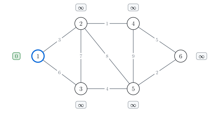
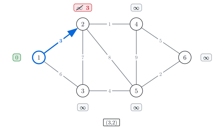
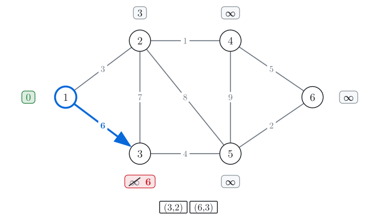
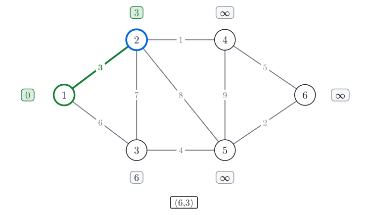
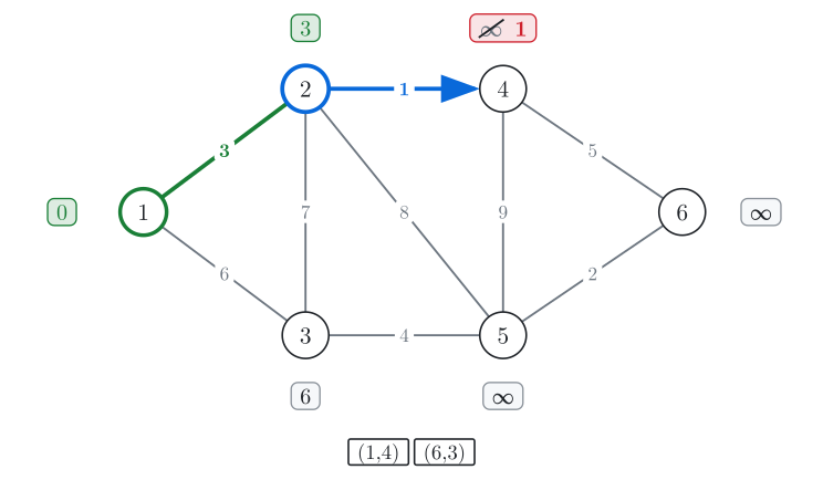
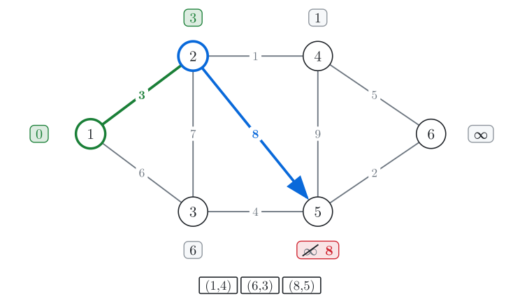
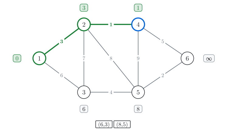
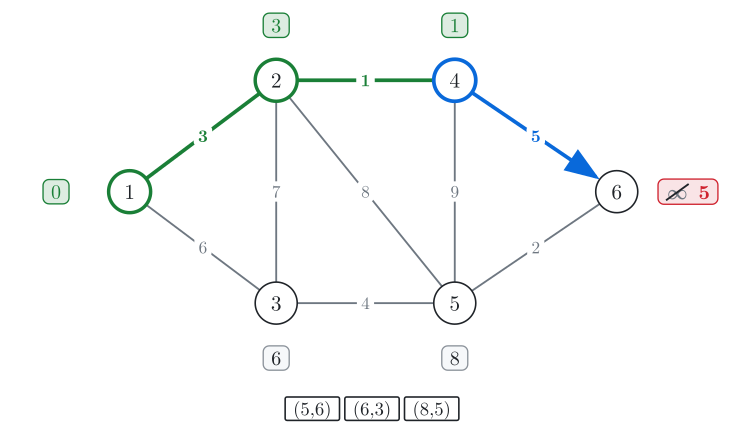
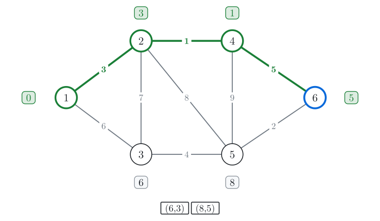
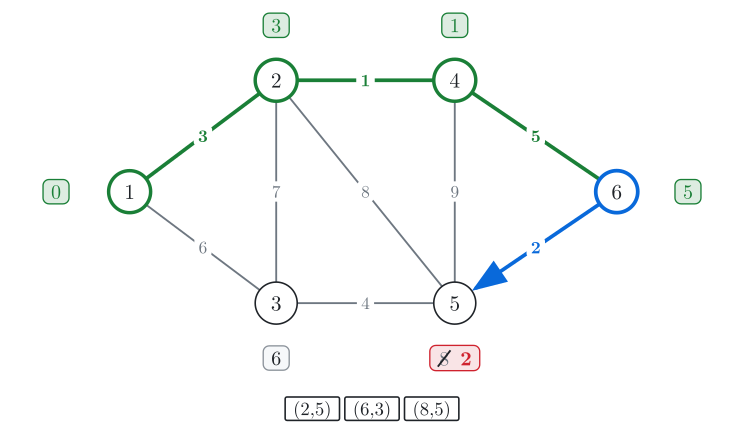
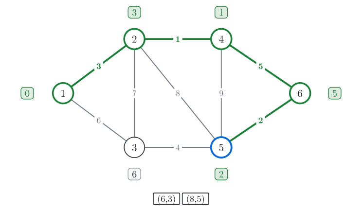
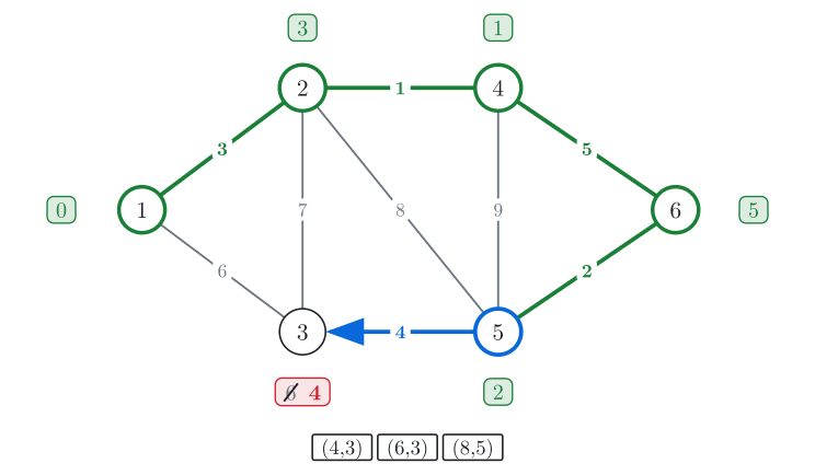
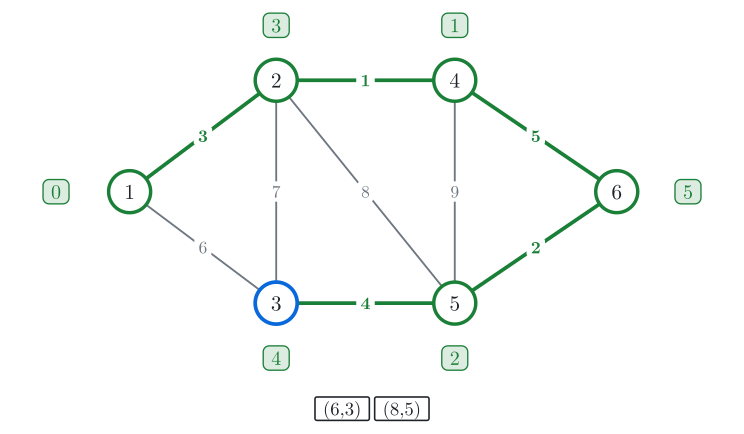
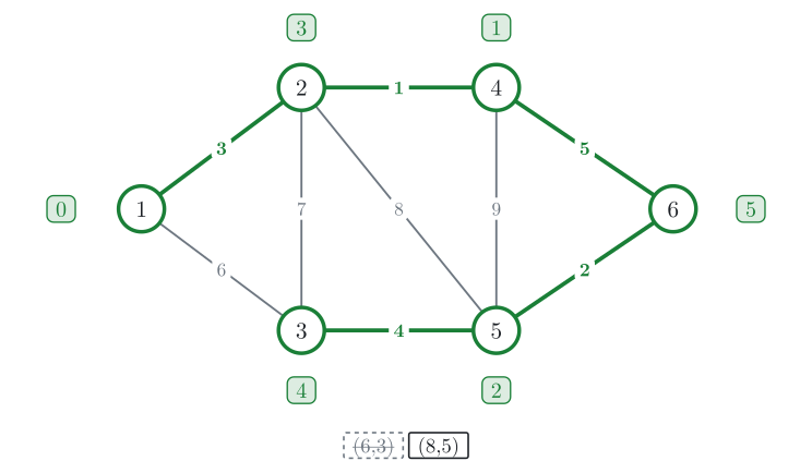
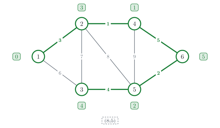
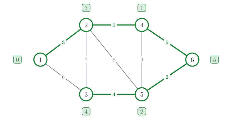
Fig. 4. Step through Prim's algorithm with the buttons. Green villages and roads are joined. The number next to a village outside is the cost of its cheapest road to a green village, and the boxes below are the priority queue.

The run paves the roads that cost 3, 1, 5, 2 and 4.

Implementation

In graph terms, villages are vertices, roads are undirected edges and costs are weights. A plan that reaches every village with no loop is a spanning tree. The joined villages and the roads that joined them form the tree. For a vertex v outside the tree, its key key[v] is the weight of its cheapest edge to the tree found so far, the number next to the village in Fig. 4. When v is added to the tree, key[v] is the weight of the edge that joins it, so total, the weight of the tree, is the sum of these keys.

The vertices outside the tree wait in the priority queue pq of pairs (key[v], v), exactly as in Dijkstra: a key that drops pushes a new pair, and the old pair becomes stale and is skipped when it comes out.

1. Initialise: key[s] = 0 for the start vertex s, every other key is INF, and the queue holds (0, s).

2. Take the next vertex v: the pair with the smallest key. If inTree[v], the pair is stale: skip it.

3. Add it to the tree: set inTree[v] = true and add key[v] to total.

4. Update the keys: for each edge v–u of weight w with !inTree[u] and w < key[u], set key[u] = w, remember parent[u] = v, and push (key[u], u).

5. Stop when the queue is empty.

If the graph is not connected, the queue empties before every vertex is in the tree, and there is no spanning tree. So we count the vertices added in added: added < n means the answer is impossible.

The program reads n and m, then m lines u v w: an undirected edge between u and v of weight w. It prints the total weight of a minimum spanning tree, or IMPOSSIBLE if the graph is not connected. Then it prints the edges of the tree, one pair per line. parent[u] is the vertex whose edge last lowered key[u]. When u is added to the tree, that edge is the one that joins it, so the tree consists of the edges parent[v]–v for every vertex v except the start. For the map of Fig. 2 the input is:

6 9
1 2 3
1 3 6
2 3 7
2 4 1
2 5 8
3 5 4
4 5 9
4 6 5
5 6 2

The graph is stored as an adjacency list adj of (neighbour, weight) pairs, and the start vertex is 1. INF is small here so that the trace is easy to follow; for real inputs, use the value in the comment.

#include <climits>
#include <iostream>
#include <queue>
#include <vector>
using namespace std;

const long long INF = 99;   // small for the demo; use LLONG_MAX for real inputs

int main() {
    int n, m;
    cin >> n >> m;
    vector<vector<pair<int, long long>>> adj(n + 1);
    for (int i = 0; i < m; i++) {
        int u, v;
        long long w;
        cin >> u >> v >> w;
        adj[u].push_back({v, w});
        adj[v].push_back({u, w});
    }

    vector<long long> key(n + 1, INF);
    vector<bool> inTree(n + 1, false);
    vector<int> parent(n + 1, 0);   // only needed to print the edges
    priority_queue<pair<long long, int>, vector<pair<long long, int>>,
                   greater<pair<long long, int>>> pq;
    long long total = 0;
    int added = 0;

    // initialise
    key[1] = 0;
    pq.push({0, 1});

    while (!pq.empty()) {              // stop: when the priority queue is empty
        // take the next vertex
        int v = pq.top().second;
        pq.pop();
        if (inTree[v]) continue;       // stale pair

        // add it to the tree
        inTree[v] = true;
        total += key[v];
        added++;

        // update the keys
        for (auto [u, w] : adj[v]) {
            if (!inTree[u] && w < key[u]) {
                key[u] = w;
                parent[u] = v;   // only needed to print the edges
                pq.push({key[u], u});
            }
        }
    }

    if (added < n) {
        cout << "IMPOSSIBLE\n";
        return 0;
    }
    cout << total << "\n";

    // print the edges of the tree; remove this block if you only need the total
    for (int v = 2; v <= n; v++) cout << parent[v] << ' ' << v << '\n';
}

On the map of Fig. 2 the program prints 15, then 1 2, 5 3, 2 4, 6 5 and 4 6, one pair per line.

Each edge pushes at most one pair from each end, so pq receives at most 2m + 1 pairs, and each push and take costs O(\log m). The total time is O(m \log m) and the memory is O(n + m), as in Dijkstra.

For a maximum spanning tree, run the same code on negated weights and negate the total.

Dense graphs

Sometimes the graph has an edge between every pair of vertices: the vertices are points on a plane, and the weight of an edge is the distance between its ends. Then m = n(n - 1)/2. For n = 10^4 the adjacency list holds 10^8 entries, more than a gigabyte.

Without the priority queue, each step scans all vertices outside the tree for the one with the smallest key. That costs $O(n)$ per step and O(n^2) in total, and the weights can be computed from the coordinates when they are needed, so no edge is stored and the memory is $O(n)$. For n = 10^4 that is 10^8 simple steps. Use this version when $m$ is close to n^2; on a sparse graph the heap version is faster.

The program reads n, then n lines with the coordinates of a point, and prints the total length of the shortest network that connects all points. For the input

4
0 0
3 0
3 4
10 0

it prints 14.00: the tree connects point 2 to the other three, with edges of length 3, 4 and 7.

#include <cmath>
#include <cstdio>
#include <iostream>
#include <vector>
using namespace std;

int main() {
    int n;
    cin >> n;
    vector<double> x(n + 1), y(n + 1);
    for (int i = 1; i <= n; i++) cin >> x[i] >> y[i];

    vector<double> key(n + 1, 1e18);
    vector<bool> inTree(n + 1, false);
    vector<int> parent(n + 1, 0);
    double total = 0;

    // initialise
    key[1] = 0;

    for (int step = 0; step < n; step++) {
        // take the next vertex: the smallest key outside the tree
        int v = 0;
        for (int u = 1; u <= n; u++)
            if (!inTree[u] && (v == 0 || key[u] < key[v])) v = u;

        // add it to the tree
        inTree[v] = true;
        total += key[v];

        // update the keys: the weight is the distance between the points
        for (int u = 1; u <= n; u++) {
            if (inTree[u]) continue;
            double w = hypot(x[u] - x[v], y[u] - y[v]);
            if (w < key[u]) {
                key[u] = w;
                parent[u] = v;
            }
        }
    }
    printf("%.2f\n", total);
}

With integer coordinates you can keep squared distances in long long as keys, which compare in the same order, and take one sqrt per tree edge when adding to the total.

Correctness proof

The algorithm keeps this invariant: the edges of the tree are part of some minimum spanning tree.

At the start the tree has no edges, so the invariant holds. Suppose it holds, the tree has the vertex set $S$, and the algorithm adds vertex $v$ by edge $e$ of weight $w$. For every vertex $u$ outside $S$, key_u is the weight of the cheapest edge from $S$ to $u$: each such edge was checked when its end in $S$ was added, and a key only goes down. Stale pairs are skipped, so the vertex taken has the smallest key outside $S$, and $e$ is a cheapest edge leaving $S$.

Let $T$ be a minimum spanning tree that contains the edges of the tree. If $T$ contains $e$, we are done. Otherwise, $T$ connects the two ends of $e$ by a path. This path starts in $S$ and ends outside it, so it leaves $S$ by some edge $f$. Remove $f$ from $T$ and add $e$. Every vertex is still connected: a path that used $f$ can use $e$ and the rest of that path instead. The weight of $e$ is at most the weight of $f$, so the new spanning tree is no heavier. It is also a minimum spanning tree, and it contains the tree and $e$. After n - 1 edges, the tree itself is a minimum spanning tree.

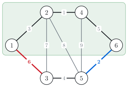
Fig. 5. The path of the spanning tree of Fig. 3 from vertex 6 to vertex 5 leaves the green region by the red edge.

In Fig. 5, $S$ holds vertices 1, 2, 4 and 6, $e$ is the blue edge, and $T$ is the spanning tree of Fig. 3. Its path from vertex 6 to vertex 5 leaves $S$ by the red edge, $f$. Swapping the two saves 6 − 2 = 4.

The proof never adds weights along a path, it only compares two single edges. So negative weights are fine for Prim, unlike for Dijkstra.

Common mistakes

• Using the distance from the start as the key, Dijkstra's update key[v] + w < key[u], which builds the shortest-route edges of Fig. 3. Compare the edge weight alone, w < key[u], and set key[u] = w.

• Not skipping stale pairs, so a vertex that comes out a second time adds its key to the total again; in Dijkstra the missing line only costs time, here it makes the answer wrong. Keep if (inTree[v]) continue;.

• Assuming the graph is connected, which prints the weight of only the part reached from the start. Count the vertices in added and print IMPOSSIBLE when added < n.

• Updating the key of a vertex already in the tree, which leaves the total right but overwrites parent, so the printed edges are wrong. Keep !inTree[u] in the update.

Similar algorithms

Dijkstra's algorithm runs the same steps with d_v + w as the key and finds the shortest routes from one vertex. Use it when the problem asks about routes from one place, and Prim when it asks only that everything be connected.

Kruskal's algorithm builds the same minimum spanning tree in another order: it sorts all edges by weight and takes each edge whose ends are in different groups of vertices, keeping the groups in a disjoint set union. On the map of Fig. 2 it takes the same five edges, in the order of their weights 1, 2, 3, 4, 5. Kruskal is shorter to write when the input is a list of edges. Prim's O(n^2) version fits complete graphs.

If all edges have the same weight, every spanning tree is a minimum one, and BFS or DFS finds one in O(n + m).

Practice