
Edge list
An edge list keeps the edges of a graph in one vector, one record per edge, usually in the order they were read. It is enough when an algorithm goes over all the edges or sorts them by weight; when it needs the neighbours of a vertex, use an adjacency list instead.
The input of most graph problems already is an edge list: n m, then m lines, one edge per line. Storing it takes no extra work and memory.
How it works
A graph has 6 vertices and 9 undirected edges, each with a weight. The edge list keeps each edge as one record of three numbers: its two ends and its weight, in the order the input gives them.
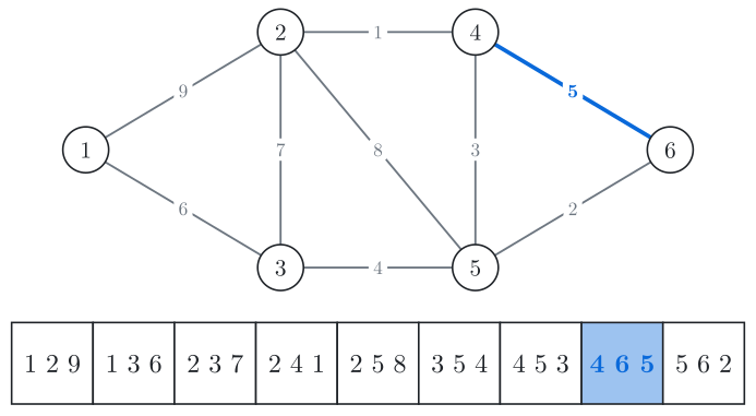
Fig. 1. One record per edge, in the order the input gives them. The edge between 4 and 6 is the record 4 6 5. An undirected edge is stored once.
Going over all edges is one pass over the records. Counting the degree of every vertex is such a pass: each record adds 1 to the degree of both its ends. Here are the degrees counted so far, after some of the records:
After the record | Vertex 1 | Vertex 2 | Vertex 3 | Vertex 4 | Vertex 5 | Vertex 6 |
|---|---|---|---|---|---|---|
| 1 | 1 | 0 | 0 | 0 | 0 |
| 2 | 2 | 2 | 0 | 0 | 0 |
| 2 | 4 | 2 | 1 | 1 | 0 |
| 2 | 4 | 3 | 2 | 3 | 0 |
| 2 | 4 | 3 | 3 | 4 | 2 |
After the last record, vertex 5 has degree 4.
Finding the neighbours of one vertex means checking every record, because its edges can be anywhere in the edge list.
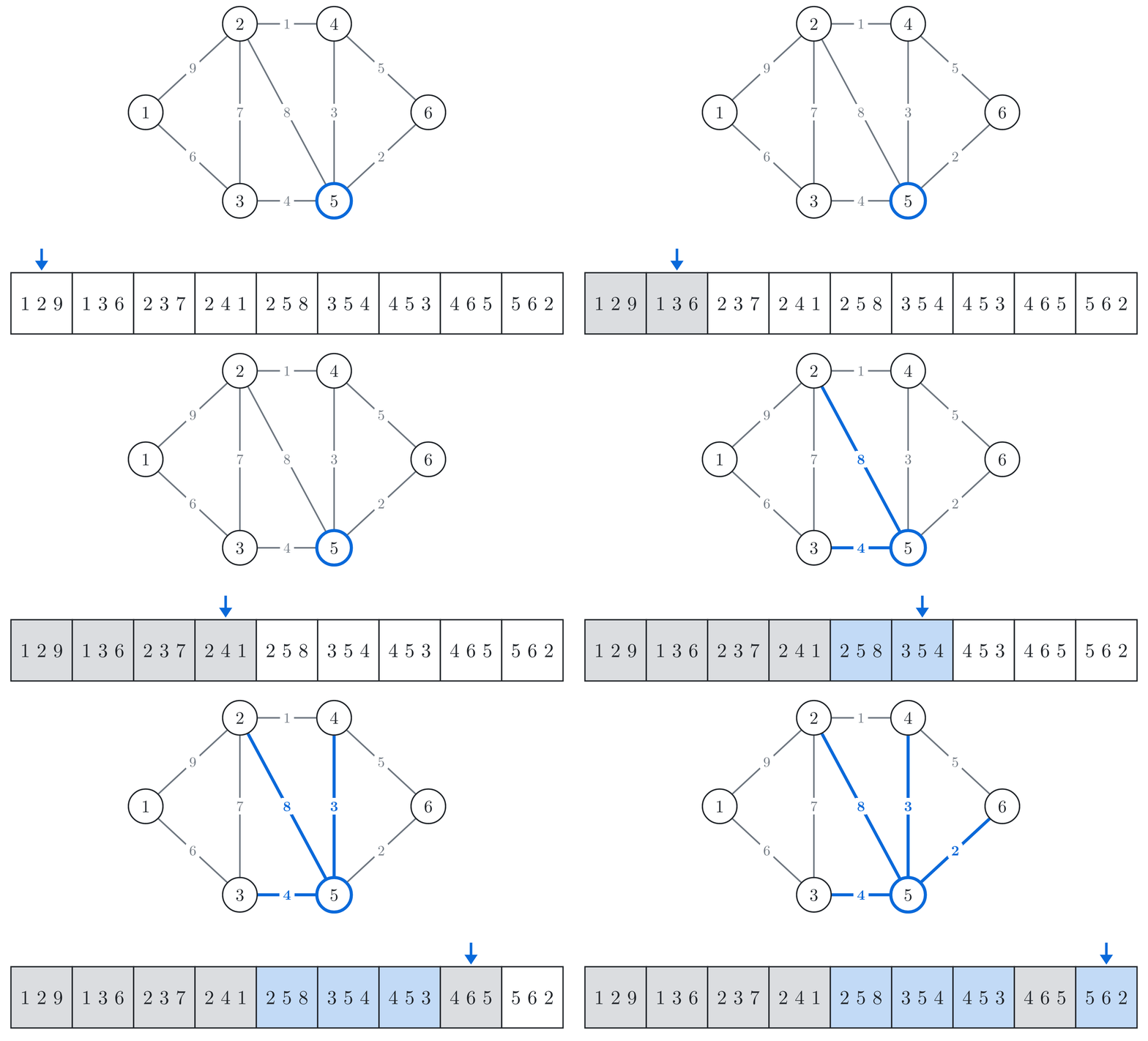
Fig. 2. To find the neighbours of vertex 5, all 9 records are checked. Four of them mention 5 (blue): its neighbours are 2, 3, 4 and 6. The 5 grey checks find nothing.
Doing this for every vertex costs 6 × 9 = 54 checks. Adjacency lists keep a list of neighbours for each vertex and write each edge into the lists of both its ends, so they give all neighbours of all vertices by reading 2 × 9 = 18 entries. Searches such as BFS and DFS ask for the neighbours of every vertex they reach, so over an edge list each step is a full scan. For them, build adjacency lists first.
All records sit in one vector, so one sort call orders them by weight, as long as each record keeps its weight first.
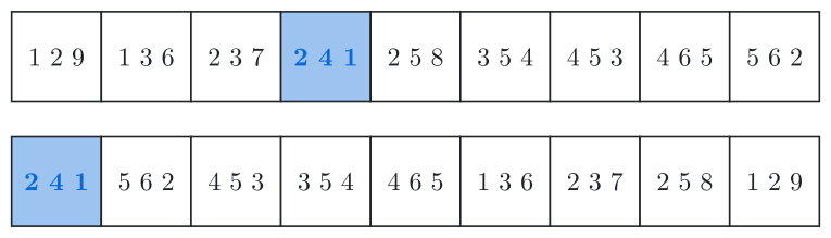
Fig. 3. The edge between 2 and 4, weight 1, moves from the fourth place to the first.
With vertices and edges, the costs in big-O notation are:
Operation | Cost |
|---|---|
Read the edges | |
Add an edge | on average |
Go over all edges | |
Sort by weight | O(m \log m) |
Find the neighbours of | |
Is there an edge between and ? | |
Memory |
In C++
The records are kept in a vector of array<int, 3>, a fixed group of three numbers that #include <array> provides. Each record is stored as {w, u, v}. sort compares two records by their first number, then by the second, then by the third, so this order sorts the edges by weight. The loop for (auto [w, u, v] : edges) (C++17) takes each record apart into its three numbers.
The program reads n and m, then m lines u v w: an undirected edge between u and v of weight w, with vertices numbered from 1. It prints the degrees, then the edges sorted by weight. For the example the input is:
6 9
1 2 9
1 3 6
2 3 7
2 4 1
2 5 8
3 5 4
4 5 3
4 6 5
5 6 2#include <algorithm>
#include <array>
#include <iostream>
#include <vector>
using namespace std;
int main() {
int n, m;
cin >> n >> m;
// read the edges
vector<array<int, 3>> edges;
for (int i = 0; i < m; i++) {
int u, v, w;
cin >> u >> v >> w;
edges.push_back({w, u, v}); // weight first: sort compares it first
}
// go over all edges: degrees
vector<int> deg(n + 1);
for (auto [w, u, v] : edges) {
deg[u]++;
deg[v]++; // remove this line to count only edges leaving u in a directed graph
}
for (int v = 1; v <= n; v++) {
cout << deg[v] << (v < n ? ' ' : '\n');
}
// sort by weight
sort(edges.begin(), edges.end());
for (auto [w, u, v] : edges) {
cout << u << ' ' << v << ' ' << w << '\n';
}
}In a directed graph, a record u v is an edge from u to v. A weight fits in int, but a sum of many weights may need long long. When the records never need sorting, a struct Edge {int u, v, w;}; also works.
Unweighted graphs
Without weights, a record is two vertices, a pair:
vector<pair<int, int>> edges;
edges.push_back({u, v});
for (auto [u, v] : edges) { /* ... */ }
Turning it into adjacency lists
When an algorithm needs the neighbours of each vertex, build adjacency lists from the records once, before the search:
vector<vector<pair<int, int>>> adj(n + 1);
for (auto [w, u, v] : edges) {
    adj[u].push_back({v, w});
    adj[v].push_back({u, w});   // remove this line if the graph is directed
}
This takes O(n + m) time: n + 1 empty lists, then one step per record.
Examples of use
Kruskal's algorithm sorts the records by weight in O(m \log m) and joins the ends of each edge with a DSU.
Bellman–Ford goes over all records in up to n - 1 rounds, O(n \cdot m) in total.
Without the sort, the same DSU pass over the records in input order counts the connected components as edges are added, with no per-vertex lists.
Common mistakes
Storing
{u, v, w}and callingsort. On the example of Fig. 1 the input is already in order of first vertex, so the list stays exactly as read: the program prints1 2 9first instead of2 4 1. Put the weight first,{w, u, v}.Reading an undirected record in one direction only, for example finding the neighbours of
xby checking onlyu == x. On Fig. 1, vertex 5 then gets the single neighbour 6, from5 6 2. It misses 2, 3 and 4, because in2 5 8,3 5 4and4 5 3vertex 5 is the second end. Check both ends of each record, or store each undirected edge as two directed records.Creating
vector<array<int, 3>> edges(m);and then callingpush_back. The edge list ends up with records, the first of them{0, 0, 0}, so a loop overedges[0]toedges[m - 1]sees only zeros, even after sorting. Either create the list empty andpush_back, or create it withmrecords and read intoedges[i].Counting pairs of joined vertices with when an edge can repeat. The records
1 2,2 1,2 3give m = 3, but only 2 pairs are joined, so a check for a complete graph on 3 vertices, m = 3 \cdot 2/2, passes although 1 and 3 are not joined. Store each pair as (smaller, larger) and sort, so equal pairs stand next to each other;uniquethen keeps one of each, and you count what is left.
Similar structures
The costs of the edge list are in the table under How it works. The other two structures give:
Adjacency list | Adjacency matrix | |
|---|---|---|
Memory | O(n + m) | O(n^2) |
Neighbours of | O(\deg v) | |
Is there an edge between and ? | O(\deg u) | |
Add an edge | on average | |
Go over all edges | O(n + m) | O(n^2) |
Sort by weight | collect the edges, then sort: O(n + m \log m) | collect the edges, then sort: O(n^2 + m \log m) |
Adjacency list
An adjacency list keeps the neighbours of each vertex together. It is the usual choice for searches such as BFS, DFS and Dijkstra's algorithm.
Adjacency matrix
An adjacency matrix is an n \times n table. It needs n^2 cells, so it fits up to about 5000 vertices: 5000^2 int cells take 100 MB.
Practice
Very easy · Implementation
Very easy · Graphs
Very easy · Shortest paths
Very easy · Disjoint set union · Graphs