Floyd–Warshall algorithm

The Floyd–Warshall algorithm finds the shortest distance between every pair of vertices of a weighted graph in $O (n^{3})$ O(n^3), so it fits graphs with up to a few hundred vertices. It allows negative edges and detects negative cycles. If you need the distances from one vertex only, use Dijkstra's algorithm or Bellman–Ford instead.

Explanation

A small town has 4 junctions joined by two-way roads, and each road has a length. Road maps often print a distance chart: a table with the shortest distance between every two junctions. We want that whole table, not the distances from one junction. Running Dijkstra's algorithm from every junction works, but each run needs a priority queue. The table itself suggests a shorter program of three loops and one line.

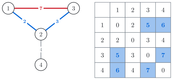
Left, a map of 4 junctions: the road from 1 to 3 of length 7 in red, the route 1–2–3 in blue with roads of length 2 and 3, and a road of length 4 from 2 to 4; right, the 4×4 table of shortest distances 0 2 5 6 / 2 0 3 4 / 5 3 0 7 / 6 4 7 0, with the six cells for pairs 1–3, 1–4 and 3–4 and their mirrors highlighted.

Fig. 1. The road between junctions 1 and 3 has length 7; the route through junction 2 has length 5. Three pairs of cells get shorter through junction 2.

The table starts with the direct roads. Junctions 1 and 3 get 7, the red road between them. Junctions 1 and 4 have no road between them, and neither do junctions 3 and 4, so their cells stay empty for now.

A route can be shorter if it passes through another junction on the way. Such a junction is a stop of the route. The blue route from 1 to 3 has one stop, junction 2, and its length is 2 + 3 = 5, less than 7. In the same way, junctions 1 and 4 get 2 + 4 = 6 through junction 2, and junctions 3 and 4 get 3 + 4 = 7. So a cell can be improved by adding two other cells: the distance to the stop and the distance on from it. In this town every shortest route has at most one stop, so trying every junction as the stop for every pair fills the table.

In a bigger town a shortest route can pass through many junctions. This one has 6 junctions and 9 roads, and we follow the pair of junctions 1 and 5.

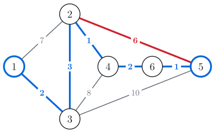
A map of 6 junctions with road lengths; junctions 1 and 5 are ringed. The blue route 1–3–2–4–6–5 has length 9. The red road 2–5 of length 6 is the other way on from junction 2, which makes the route 1–3–2–5 of length 11.

Fig. 2. Find the shortest distance between junctions 1 and 5. The blue route has four stops. The red route follows it as far as junction 2 and then takes the red road.

The blue route has length 2 + 3 + 1 + 2 + 1 = 9. With only one stop, the best is 2 + 10 = 12, through junction 3.

Fill the table in reading order, row by row, and for each pair try every junction as the stop, using the numbers already in the table, including the ones improved a moment ago. This does build routes with several stops. By the time we reach junctions 1 and 4, the cell for 1 and 2 already holds 5, through junction 3. So junctions 1 and 4 get 5 + 1 = 6, a route with two stops.

For junctions 1 and 5, the best sum the table offers is 5 + 6 = 11, through junction 2: the red route. The blue route needs one of two cells that are still empty (Fig. 3). Through junction 6 it would add the distance from 1 to 6, which is 8, but that cell is filled right after the cell for 1 and 5. Through junction 4 it would add the distance from 4 to 5, which is 3, but row 4 comes much later. Repeating the whole pass does fix it: the second pass finds 9. But there is an order in which one pass is enough.

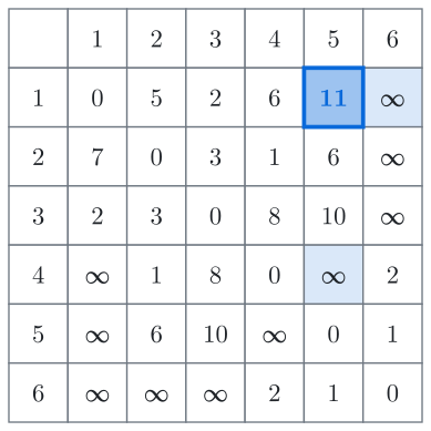
A 6 by 6 distance table for junctions 1 to 6, filled row by row and stopped at the cell for junctions 1 and 5, which holds 11 and is highlighted; the cells for 1 and 6 and for 4 and 5 are shaded and still hold infinity.

Fig. 3. Filled in reading order, the cell for junctions 1 and 5 gets 11. The cells 1–6 and 4–5, which would give 8 + 1 = 9 and 6 + 3 = 9, are still empty.

A cell is built from two other cells, and those must already be right for the routes we try. Look at the blue route again. Of its stops, junction 6 has the largest number. It splits the route into two parts: from 1 to 6, of length 8, and from 6 to 5, of length 1. Neither part stops at junction 6 or above: they stop only at junctions 2, 3 and 4. So if the table already held the shortest routes that stop only at junctions 1 to 5, one addition, 8 + 1, would give 9. The part from 1 to 6 splits in the same way at its own largest stop, junction 4, and so on down.

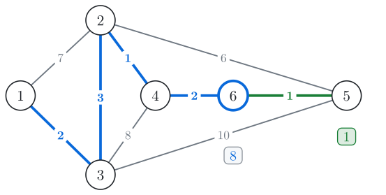
The shortest route from junction 1 to junction 5, 1-3-2-4-6-5, split at junction 6: the blue part from 1 to 6 has length 8, shown in a tag under junction 6, and the green part from 6 to 5 has length 1, shown in a tag under junction 5.

Fig. 4. Junction 6 is the stop of the blue route with the largest number. The two parts have lengths 8 and 1, and they stop only at junctions 2, 3 and 4.

That suggests an order. At first no stops are allowed. The table holds the direct roads, and that is right for routes without stops. Then junction 1 is allowed as a stop, then junctions 1 and 2, and so on, one junction per round. When a new junction is allowed, take a shortest route that may stop at it. Either it doesn't stop there, and its length is already in the cell, or it passes through the new junction once. In that case the part before the new junction and the part after it stop only at junctions allowed earlier, so their lengths are already in the table. Each cell needs one addition: compare it with the distance to the new junction plus the distance on from it. So after each round, every cell holds the shortest route that stops only at the junctions allowed so far.

The cell for junctions 1 and 5 gets 7 + 6 = 13 when junction 2 is allowed. It gets 2 + 9 = 11 when junction 3 is allowed, where 9 is the distance from 3 to 5 through junction 2. It gets 8 + 1 = 9 when junction 6 is allowed, the last round.

This is the Floyd–Warshall algorithm. Each round relaxes every pair through the new stop: it tries the stop and keeps the sum if it is shorter. In this town that is 6 rounds, and each round checks all 36 cells.

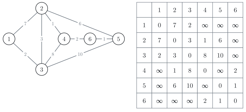
Floyd–Warshall on the 6-junction town, step 1.

The table starts with the direct roads. No stops are allowed yet, and pairs without a road hold ∞.

1/23

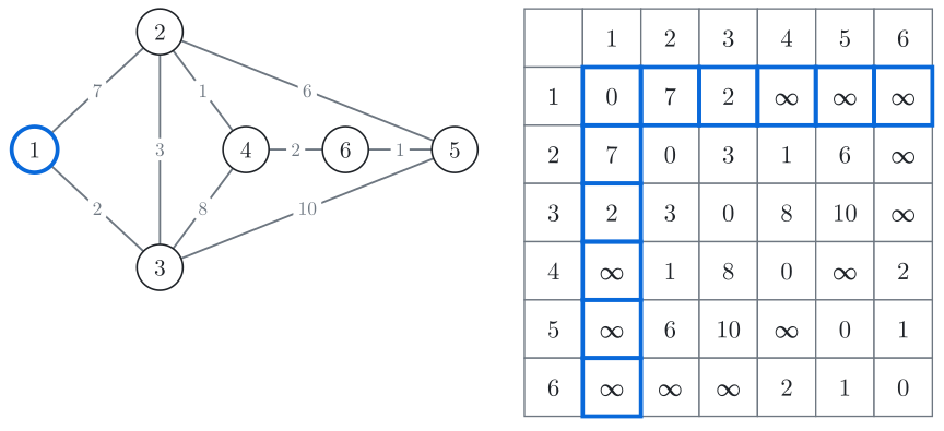
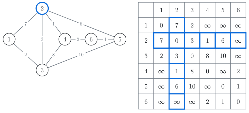
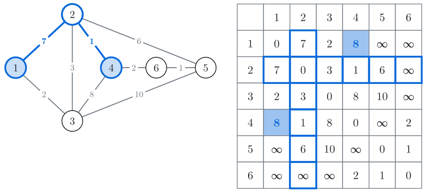
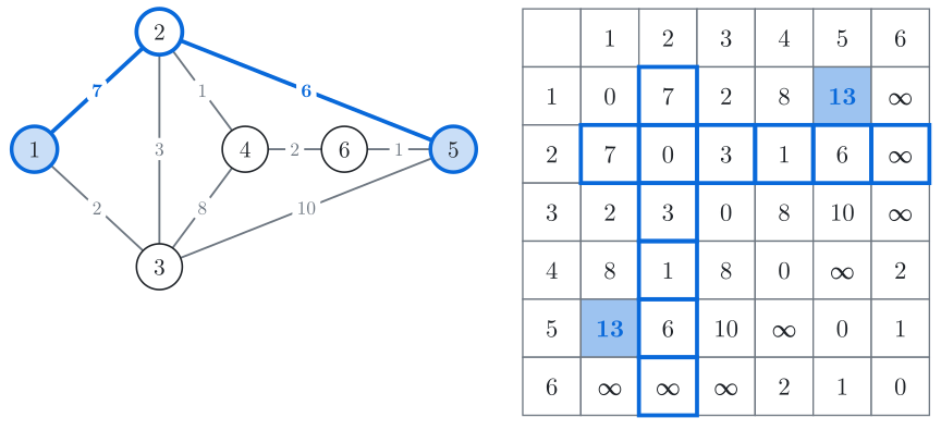
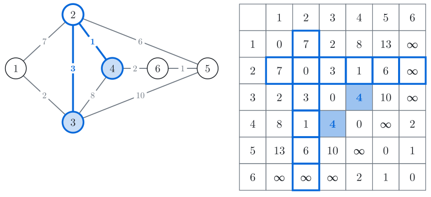
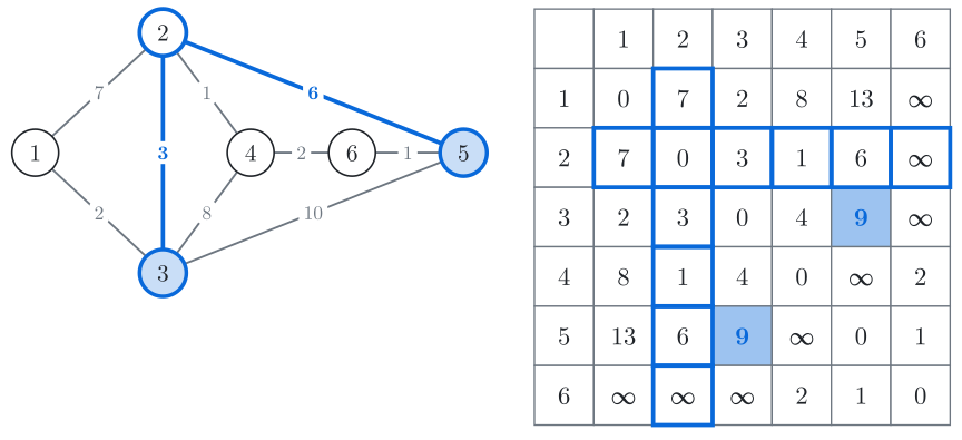
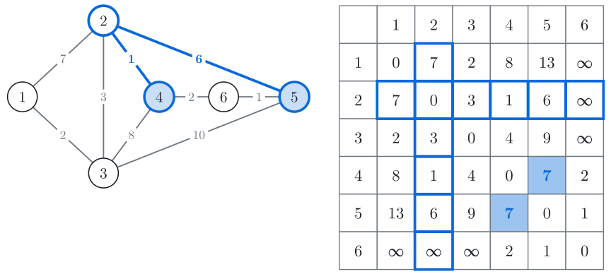
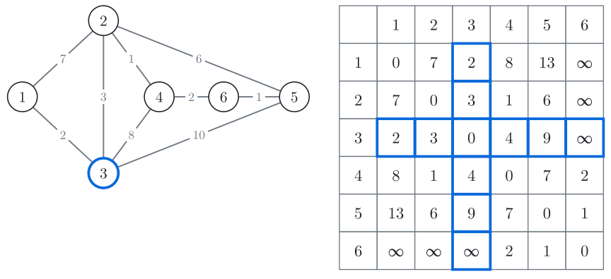
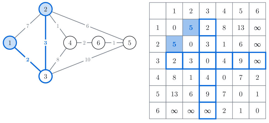
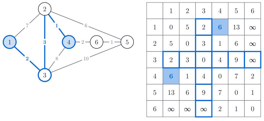
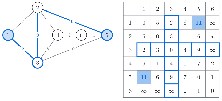
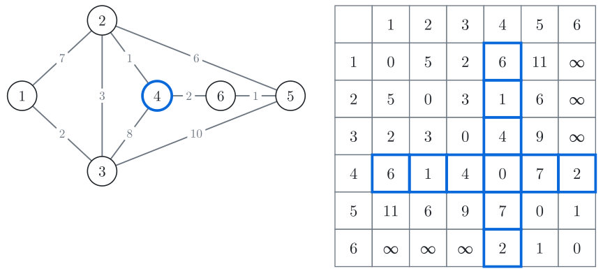
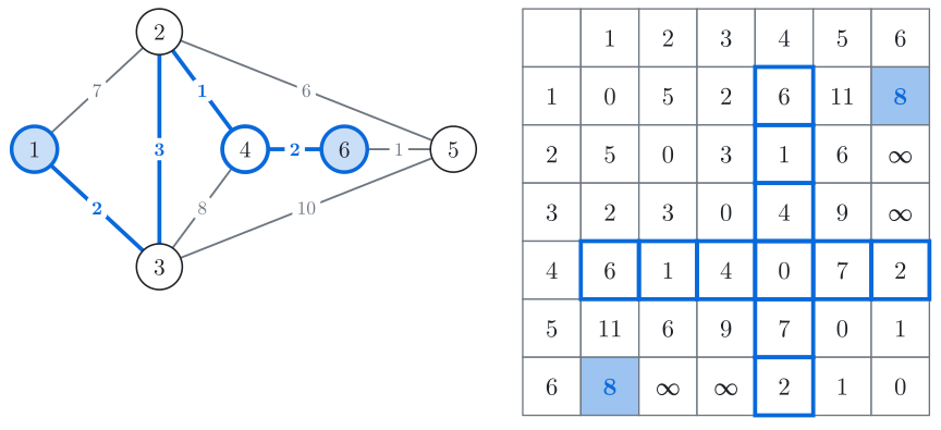
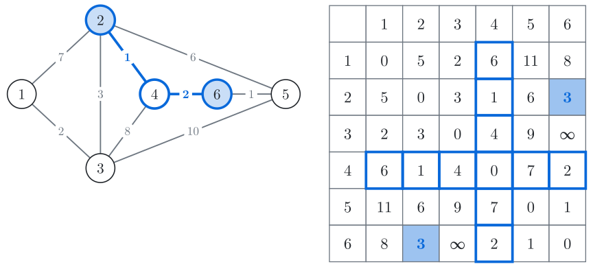
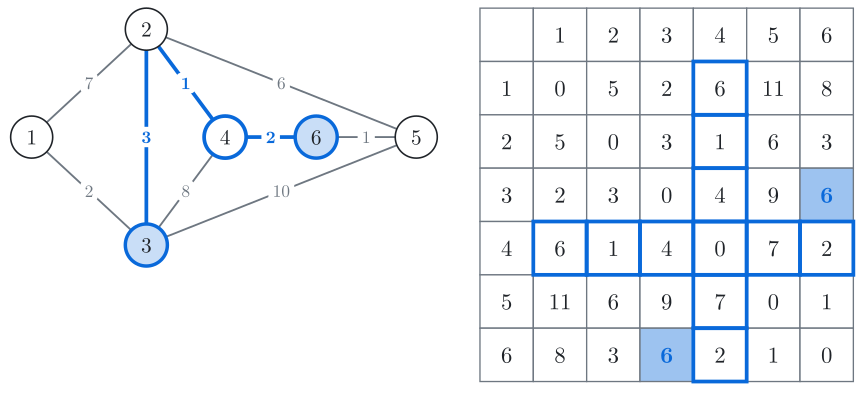
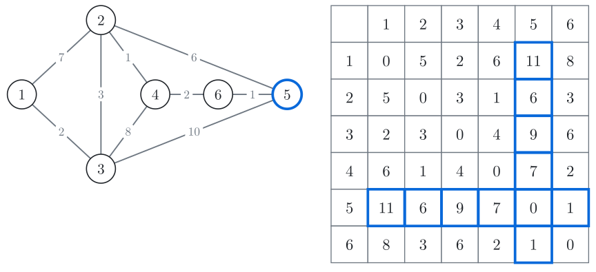
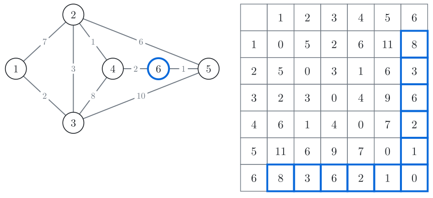
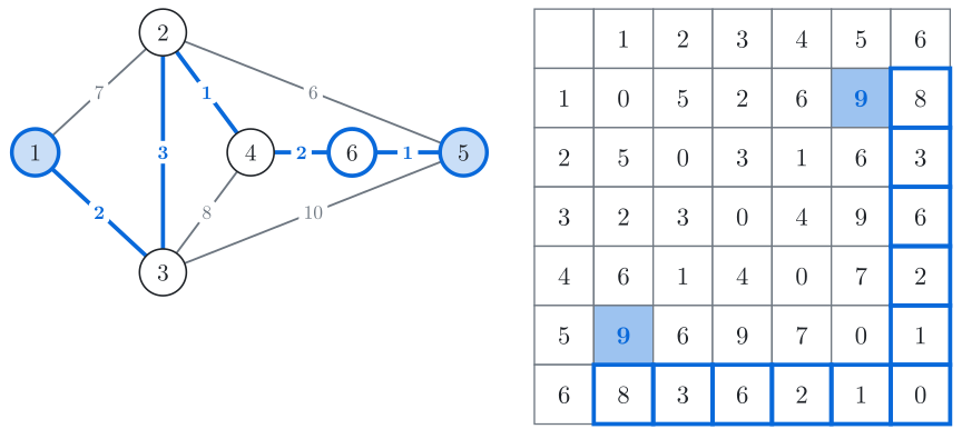
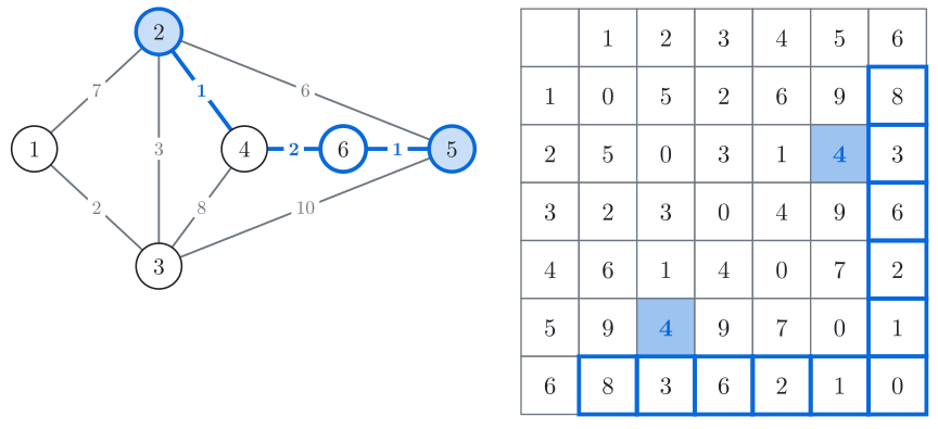
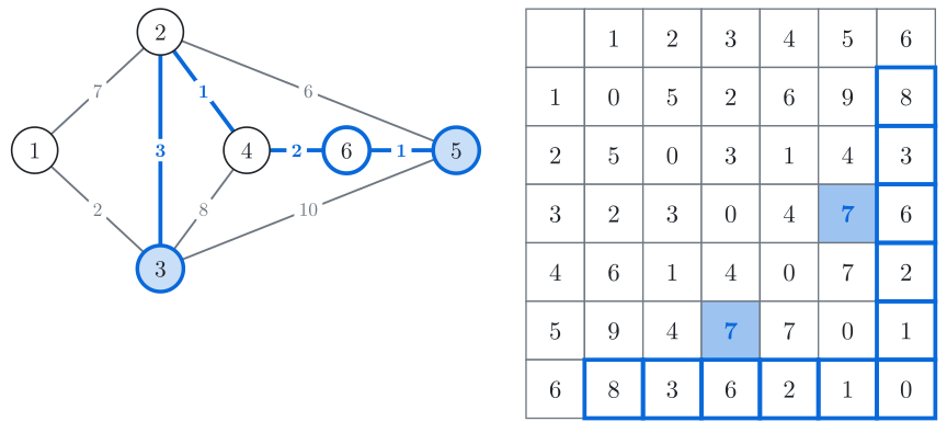
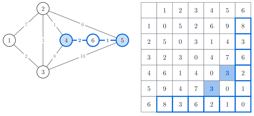
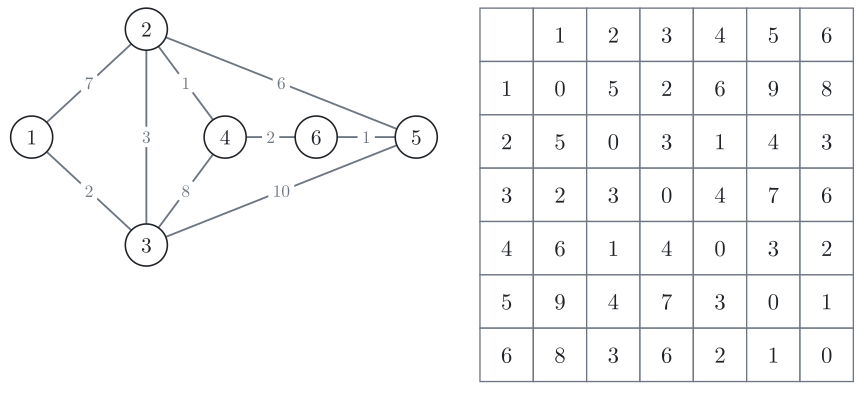
Fig. 5. Step through Floyd–Warshall with the buttons. The ringed junction is the new stop, its row and column of the table are framed, and the blue route goes through it. A cell changes when that route is shorter.

The shortest distance between junctions 1 and 5 is 9. The row of junction 1, 0, 5, 2, 6, 9, 8, is exactly what Dijkstra's algorithm computes from junction 1, and every other row came from the same run.

In graph terms, junctions are vertices, roads are edges, and routes are paths. A road's length is the weight of its edge, and the length of a path is the sum of its weights. A stop is an intermediate vertex of a path: any vertex of the path except its two ends. Let $d_{ij}$ d_{ij} be the number in row $i$ and column $j$ of the table.

Negative edges and negative cycles

Negative weights make sense only on a directed graph: a two-way edge $u$ – $v$ of weight $w < 0$ w < 0 is itself the cycle $u \to v \to u$ u \to v \to u of length $2 w$ . On a directed graph Floyd–Warshall works unchanged with negative weights, as long as no cycle has negative length. The argument above never used that weights are positive, only that a shortest path passes through each vertex at most once. Take the graph in Fig. 6.

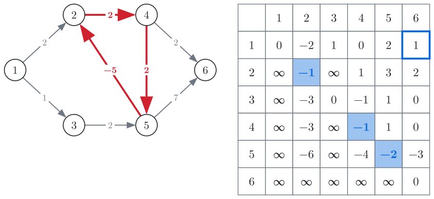
A directed graph of 6 vertices with the cycle 2→4→5→2 (weights 2, 2 and −5, total −1) in red, beside its final 6×6 distance table, where the diagonal cells of vertices 2, 4 and 5 are highlighted (−1, −1, −2) and the cell from 1 to 6, holding 1, is framed.

Fig. 6. The red cycle has length −1. Vertices 2, 4 and 5 end with negative numbers on the diagonal.

First give the edge $5 \to 2$ 5 \to 2 the weight −3 instead of −5. The run gives the row 0, 0, 1, 2, 3, 4 for vertex 1, the same distances Bellman–Ford finds from vertex 1. For example, $d_{12} = 0$ d_{12} = 0 along the path through vertices 3 and 5: 1 + 2 − 3.

Every $d_{ii}$ d_{ii} starts at 0: the path from $i$ to itself that doesn't move. Give the edge $5 \to 2$ 5 \to 2 the weight −5, as in Fig. 6. The red cycle has length 2 + 2 − 5 = −1, a negative cycle: each trip around it makes a path shorter. After the run, $d_{22} = - 1$ d_{22} = -1, $d_{44} = - 1$ d_{44} = -1 and $d_{55} = - 2$ d_{55} = -2. A vertex on a negative cycle has a path of negative length back to itself, so it ends with a negative number on the diagonal. The value itself means only "below zero": −2 at vertex 5 is not the length of the cycle.

The other cells can be wrong too. $d_{16} = 1$ d_{16} = 1 looks like an answer, but a path from 1 to 6 can go around the cycle as many times as it likes, so no path is the shortest. The same holds for every pair whose paths can pass through the cycle: in Fig. 6 these are the 20 pairs with $i$ among vertices 1 to 5 and $j$ among vertices 2, 4, 5 and 6. In general, the pair $(i, j)$ has no shortest path when some $k$ has $d_{ik} < \infty$ d_{ik} < \infty, $d_{k j} < \infty$ d_{kj} < \infty and $d_{k k} < 0$ d_{kk} < 0. Bellman–Ford only sees the negative cycles it can reach from its start, while this check finds every negative cycle in the graph.

Implementation

d[i][j] is the length of the shortest path from i to j found so far, with vertices numbered from 1 to n.

Initialise d as the adjacency matrix of the graph: d[i][i] = 0; d[u][v] is the smallest weight among the edges from u to v; every other cell is INF.
Allow intermediate vertex k: rounds k = 1, ..., n.
Relax every pair through k: for every i and j with d[i][k] != INF and d[k][j] != INF, if d[i][k] + d[k][j] < d[i][j], set d[i][j] = d[i][k] + d[k][j].
Check the diagonal: a negative d[i][i] means a negative cycle through i.

To print a shortest path, the program keeps a second table: nxt[i][j] is the first vertex after i on the shortest path from i to j found so far. For an edge from u to v it is v, and nxt[i][i] = i. Cells with no path are never read. When the pair (i, j) improves through k, the new path starts like the path from i to k, so nxt[i][j] = nxt[i][k]. To print the path from s to t, start at s and follow nxt towards t.

The program reads n and m, then m lines u v w: a two-way edge between u and v of weight w. It prints negative cycle if there is one. Otherwise it prints the table, with * for a pair that has no path, since −1 can be a real distance when edges are negative, and then the shortest path from vertex s = 1 to vertex t = 5. For the 6-vertex graph of Fig. 2 the input is:

INF is small here so that the trace is easy to follow; for real inputs, use the value in the comment.

#include <iostream>
#include <vector>
using namespace std;

const long long INF = 99;   // small for the demo; use 1e18 for real inputs

int main() {
    int n, m;
    cin >> n >> m;

    // initialise
    vector<vector<long long>> d(n + 1, vector<long long>(n + 1, INF));
    vector<vector<int>> nxt(n + 1, vector<int>(n + 1, 0));   // only needed to print the path
    for (int i = 1; i <= n; i++) {
        d[i][i] = 0;
        nxt[i][i] = i;   // only needed to print the path
    }
    for (int e = 0; e < m; e++) {
        int u, v;
        long long w;
        cin >> u >> v >> w;
        if (w < d[u][v]) {
            d[u][v] = w;
            nxt[u][v] = v;   // only needed to print the path
        }
        // remove this block if the graph is directed
        if (w < d[v][u]) {
            d[v][u] = w;
            nxt[v][u] = u;   // only needed to print the path
        }
    }

    // allow intermediate vertex k
    for (int k = 1; k <= n; k++) {
        // relax every pair through k
        for (int i = 1; i <= n; i++) {
            if (d[i][k] == INF) continue;
            for (int j = 1; j <= n; j++) {
                if (d[k][j] == INF) continue;
                if (d[i][k] + d[k][j] < d[i][j]) {
                    d[i][j] = d[i][k] + d[k][j];
                    nxt[i][j] = nxt[i][k];   // only needed to print the path
                }
            }
        }
    }

    // check the diagonal
    for (int i = 1; i <= n; i++) {
        if (d[i][i] < 0) {
            cout << "negative cycle\n";
            return 0;
        }
    }

    for (int i = 1; i <= n; i++) {
        for (int j = 1; j <= n; j++) {
            if (d[i][j] == INF) cout << '*';
            else cout << d[i][j];
            cout << (j < n ? ' ' : '\n');
        }
    }

    // print the shortest path from s to t; remove this block if you only need distances
    int s = 1, t = 5;
    if (d[s][t] != INF) {
        for (int v = s; v != t; v = nxt[v][t]) cout << v << ' ';
        cout << t << '\n';
    }
}

C++

From vertex 1 to vertex 5 the run leaves nxt[1][5] = 3, nxt[3][5] = 2, nxt[2][5] = 4, nxt[4][5] = 6 and nxt[6][5] = 5, so the program prints the path 1 3 2 4 6 5, the blue route of Fig. 2. Since the edges here are two-way, the program reports a negative cycle for any negative edge, as it should.

There are $n$ rounds of $n^{2}$ n^2 pairs, so the time is $O (n^{3})$ O(n^3) and the memory is $O (n^{2})$ O(n^2), whatever the number of edges.

Which line completes the relaxation, so that the path can be printed?

if (d[i][k] + d[k][j] < d[i][j]) {
    d[i][j] = d[i][k] + d[k][j];
    // your line here
}

nxt[i][j] = nxt[i][k];

nxt[i][j] = k;

nxt[i][j] = nxt[k][j];

Reachability and other path measures

The three loops work with other ways of combining paths. To know only which pairs are connected (problem 10157), keep a table of true and false, starting with true on the diagonal and for each edge. A path from i to j exists if one existed before, or if i reaches k and k reaches j:

reach[i][j] = reach[i][j] || (reach[i][k] && reach[k][j]);

A truck can carry over a path only as much as its weakest edge allows. To find the path whose weakest edge is the strongest (problem 4114), let cap[i][j] be the best load found so far: a very large number on the diagonal, the edge's limit for an edge, 0 where there is no edge. Replace the sum by min and the comparison by max:

cap[i][j] = max(cap[i][j], min(cap[i][k], cap[k][j]));

With exchange rates, converting money along a path multiplies the rates (problem 6664). Start with 1 on the diagonal, the rate for each edge and 0 elsewhere, keep the best product found so far, and replace the sum by a product. A diagonal cell greater than 1 means a cycle of exchanges that ends with more money than it started with:

r[i][j] = max(r[i][j], r[i][k] * r[k][j]);

Correctness proof

The algorithm keeps this invariant: after round $k$ , $d_{ij}$ d_{ij} is the length of the shortest path from $i$ to $j$ whose intermediate vertices are all among $1, \dots, k$ 1, \dots, k. We assume no negative cycle, so such a shortest path visits each vertex at most once.

Before round 1, no intermediate vertex is allowed, and the table holds exactly the edges, so the invariant holds for $k = 0$ k = 0. Suppose it holds after round $k - 1$ k - 1, and take the shortest path from $i$ to $j$ with intermediate vertices among $1, \dots, k$ 1, \dots, k. If $k$ is not on it, its length is already $d_{ij}$ d_{ij}. If $k$ is on it, $k$ appears once and splits it into a path from $i$ to $k$ and a path from $k$ to $j$ , as Fig. 4 shows for $k = 6$ k = 6. The intermediate vertices of both parts are among $1, \dots, k - 1$ 1, \dots, k - 1, so after round $k - 1$ k - 1, $d_{ik}$ d_{ik} and $d_{k j}$ d_{kj} are at most their lengths. The relaxation through $k$ makes $d_{ij} \leq d_{ik} + d_{k j}$ d_{ij} \le d_{ik} + d_{kj}, which is at most the length of the path. Every value in the table is the length of a real path, so it never drops below the shortest one. After round $n$ every vertex is allowed, and $d_{ij}$ d_{ij} is the shortest distance.

The step used the values of $d_{ik}$ d_{ik} and $d_{k j}$ d_{kj} after round $k - 1$ k - 1, while the code reads them from the same table that round $k$ is changing, so one table is enough. They are the same values: a relaxation of $d_{ik}$ d_{ik} through $k$ compares it with $d_{ik} + d_{k k} = d_{ik}$ d_{ik} + d_{kk} = d_{ik}, so row $k$ and column $k$ don't change in round $k$ . With a negative cycle $d_{k k}$ d_{kk} can be negative, but then the run only has to detect the cycle.

Common mistakes

Putting the loop over k inside, so each cell is computed once, in reading order as in Fig. 3, and a cell that needs a cell filled later stays wrong. Keep the loop over k outermost.
Reading an edge as d[u][v] = w, so a later, heavier edge between the same vertices overwrites the lighter one and an edge from a vertex to itself overwrites d[i][i] = 0. Keep the smaller weight, as the program does with if (w < d[u][v]), in both directions for a two-way edge.
Adding INF to a number, which overflows int and can report a negative cycle that doesn't exist, or with negative edges turns "no path" into something that looks like a distance. Skip such cells with the two continue lines and keep d in long long, as the code above does.
Thinking a negative cycle spoils only the diagonal, though in Fig. 6 $d_{16} = 1$ d_{16} = 1 is not a distance either. Mark every pair $(i, j)$ that can pass through a vertex with a negative diagonal cell, as in Negative edges and negative cycles (problem 976).

Similar algorithms

Dijkstra's algorithm finds the distances from one vertex when no weight is negative. Run from every vertex, it gives all pairs in $O (n (n + m) lo g m)$ O(n (n + m) \log m). That is better for a sparse graph with $n$ in the thousands. For a dense graph, where $m$ is close to $n^{2}$ n^2, it is slower than Floyd–Warshall and longer to write.

Bellman–Ford finds the distances from one vertex with negative edges in $O (nm)$ . Run from every vertex it would cost $O (n^{2} m)$ O(n^2 m).

If every edge has the same weight, BFS from every vertex gives all pairs in $O (n (n + m))$ O(n (n + m)). The same works for reachability when $n$ is too large for $O (n^{3})$ O(n^3), as in problem 3330.

Johnson's algorithm runs Bellman–Ford once to make all weights non-negative, then Dijkstra from every vertex. It is for sparse graphs with negative edges.

Practice

Problem 974 gives the graph as a matrix, not a list of edges.

Floyd - 1#974

Easy · Dynamic programming · Shortest paths · Graphs

Diameter of the graph#1796

Medium · Shortest paths · Graphs

Stockbroker Grapevine#3219

Medium · Shortest paths · Graphs

Transitive closure#10157

Medium · Depth-first Search · Graphs

Floyd - existence#976

Easy · Graphs

Heavy Cargo#4114

Very easy · Graphs · Shortest paths

Arbitrage#6664

Medium · Shortest paths · Graphs

Pink Floyd#2966

Easy · Graphs

Moortal Kombat#10292

Hard · Prefix Sums

Transitive Closure#3330

Very easy · Graphs

Was this page helpful?